AP Statistics Flashcards: Least Squares Regression

What this deck covers

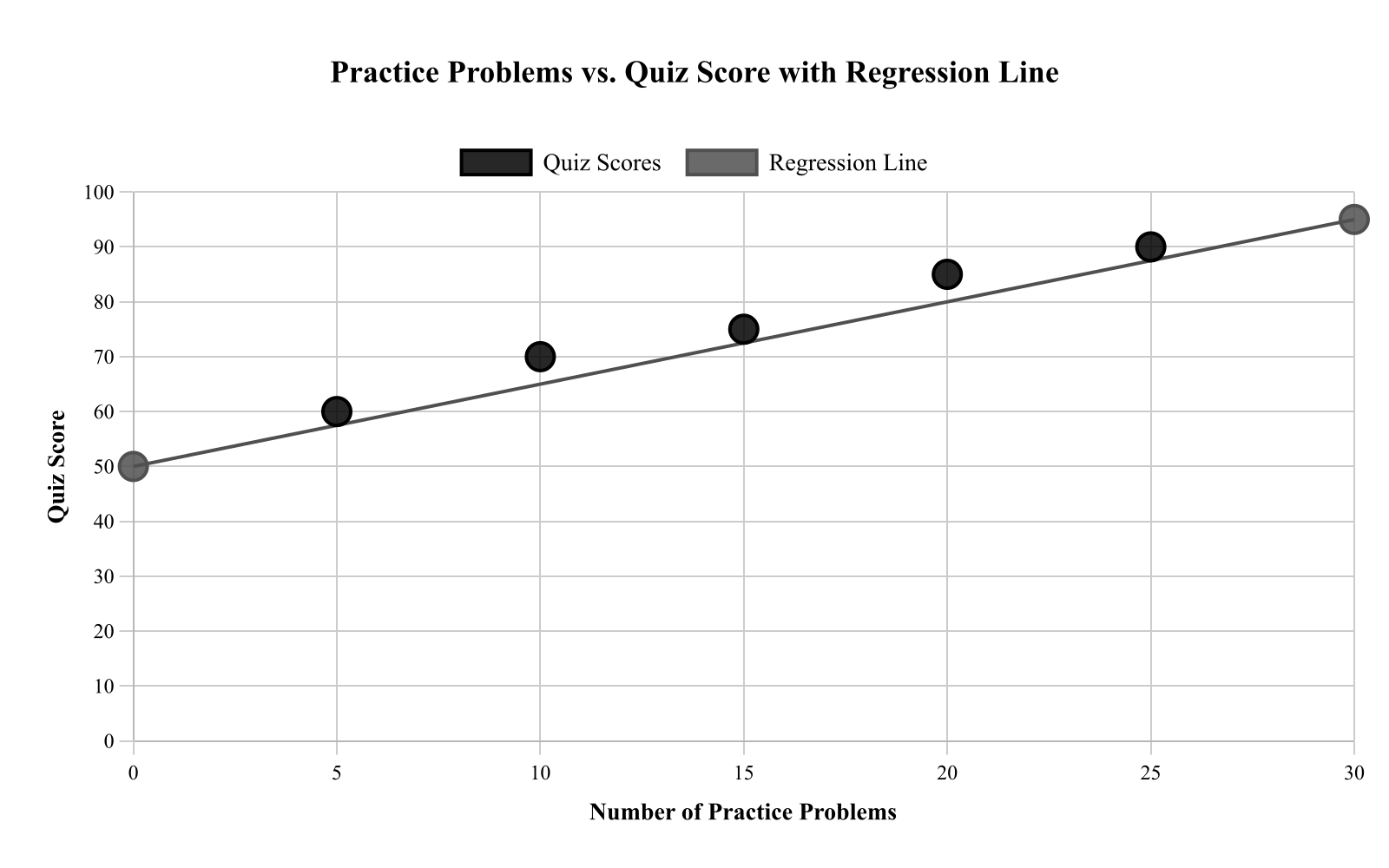
This deck focuses on Least Squares Regression, giving you a quick way to review the definitions, rules, and examples that matter most for AP Statistics.

How to use these flashcards

Work through these flashcards in short sessions. Try to answer each prompt before flipping the card, then revisit any cards you miss until the explanation feels automatic.

Flashcard 1: Identify the formula for calculating the correlation coefficient $r$.

Answer: $r = \frac{\sum (x_i - \bar{x})(y_i - \bar{y})}{\sqrt{\sum (x_i - \bar{x})^2 \sum (y_i - \bar{y})^2}}$. Standardized covariance measuring linear association strength.

Flashcard 2: In regression, what is the significance of a horizontal line as the regression line?

Answer: No linear relationship between variables. Slope is zero when variables are uncorrelated.

Flashcard 3: Which type of plot is used to assess residuals in regression?

Answer: Residual plot. Plots residuals vs. fitted values or explanatory variable.

Flashcard 4: What is the objective of least squares regression?

Answer: Minimize the sum of squared residuals. Finds line that best fits data by minimizing prediction errors.

Flashcard 5: In least squares regression, what does $b$ represent?

Answer: Slope of the regression line. Rate of change in $y$ per unit change in $x$.

Flashcard 6: What does a negative slope indicate in a regression line?

Answer: Negative relationship between variables. As $x$ increases, $y$ tends to decrease.

Flashcard 7: Identify the formula for the regression sum of squares $SS_{reg}$.

Answer: $SS_{reg} = \sum (\hat{y}_i - \bar{y})^2$. Variation in predicted values around mean of $y$.

Flashcard 8: What condition does the normal probability plot of residuals check?

Answer: Normality of residuals. Tests if residuals follow normal distribution.

Flashcard 9: What is the primary assumption about errors in least squares regression?

Answer: Errors are normally distributed. Required for valid inference and prediction intervals.

Flashcard 10: What does a positive slope indicate in a regression line?

Answer: Positive relationship between variables. As $x$ increases, $y$ tends to increase.

Flashcard 11: Identify the formula for the residual sum of squares $SS_{res}$.

Answer: $SS_{res} = \sum (y_i - \hat{y}_i)^2$. Variation not explained by the regression model.

Flashcard 12: What is the purpose of transforming variables in regression?

Answer: To achieve linearity. Makes curved relationships appear linear.

Flashcard 13: In regression, what is the significance of a horizontal line as the regression line?

Answer: No linear relationship between variables. Slope is zero when variables are uncorrelated.

Flashcard 14: What does it mean if $R^2 = 1$ in regression analysis?

Answer: Perfect explanatory power in the model. Model explains all variation in $y$ perfectly.

Flashcard 15: What does a residual plot showing random scatter indicate?

Answer: Appropriate model for the data. Random scatter indicates model assumptions are met.

Flashcard 16: What is the formula for the least squares regression line?

Answer: $y = a + bx$. Standard form where $a$ is intercept and $b$ is slope.

Flashcard 17: In least squares regression, what does $a$ represent?

Answer: Y-intercept of the regression line. Value of $y$ when $x = 0$.

Flashcard 18: What is the condition of homoscedasticity in regression?

Answer: Constant variance of residuals. Residual spread remains constant across all fitted values.

Flashcard 19: What is the purpose of transforming variables in regression?

Answer: To achieve linearity. Makes curved relationships appear linear.

Flashcard 20: State the condition for using least squares regression.

Answer: Linear relationship between variables. Assumes straight-line relationship exists.

Flashcard 21: Find the intercept $a$ given $\bar{y} = 10$, $b = 2$, and $\bar{x} = 3$.

Answer: $a = 4$. Using formula $a = 10 - (2)(3) = 4$.

Flashcard 22: What does the term 'extrapolation' refer to in regression?

Answer: Predicting outside the range of the data. Risky because relationships may change outside observed range.

Flashcard 23: Find the slope of the regression line given $\sum (x_i - \bar{x})(y_i - \bar{y}) = 10$ and $\sum (x_i - \bar{x})^2 = 5$.

Answer: $b = 2$. Using formula $b = \frac{10}{5} = 2$.

Flashcard 24: What does $R^2$ represent in regression analysis?

Answer: Proportion of variance explained by the model. Coefficient of determination; ranges from 0 to 1.

Flashcard 25: What is the formula for the least squares regression line?

Answer: $y = a + bx$. Standard form where $a$ is intercept and $b$ is slope.

Flashcard 26: How do you interpret a residual plot that shows a pattern?

Answer: Model may not be appropriate. Patterns suggest violations of linearity assumption.

Flashcard 27: What is the effect of an outlier on a regression line?

Answer: Can significantly alter slope and intercept. Outliers pull the line toward themselves disproportionately.

Flashcard 28: Find the slope of the regression line given $\sum (x_i - \bar{x})(y_i - \bar{y}) = 10$ and $\sum (x_i - \bar{x})^2 = 5$.

Answer: $b = 2$. Using formula $b = \frac{10}{5} = 2$.

Flashcard 29: Identify the formula for the regression sum of squares $SS_{reg}$.

Answer: $SS_{reg} = \sum (\hat{y}_i - \bar{y})^2$. Variation in predicted values around mean of $y$.

Flashcard 30: Identify the formula for calculating the slope $b$ in regression.

Answer: $b = \frac{\sum (x_i - \bar{x})(y_i - \bar{y})}{\sum (x_i - \bar{x})^2}$. Covariance divided by variance of $x$.

Flashcard 31: What does $R^2$ represent in regression analysis?

Answer: Proportion of variance explained by the model. Coefficient of determination; ranges from 0 to 1.

Flashcard 32: What is the effect of heteroscedasticity in regression?

Answer: Non-constant variance of residuals. Residual spread changes systematically with fitted values.

Flashcard 33: What does the term 'least squares' refer to in regression?

Answer: Minimizing the sum of squared residuals. Method minimizes sum of squared prediction errors.

Flashcard 34: What is the effect of a high leverage point in regression?

Answer: Can disproportionately influence the regression line. Points far from $\bar{x}$ have greater impact.

Flashcard 35: What is the effect of a high leverage point in regression?

Answer: Can disproportionately influence the regression line. Points far from $\bar{x}$ have greater impact.

Flashcard 36: What is the objective of least squares regression?

Answer: Minimize the sum of squared residuals. Finds line that best fits data by minimizing prediction errors.

Flashcard 37: Which term describes the strength and direction of a linear relationship?

Answer: Correlation coefficient. Ranges from -1 to +1, denoted by $r$.

Flashcard 38: Which term describes the strength and direction of a linear relationship?

Answer: Correlation coefficient. Ranges from -1 to +1, denoted by $r$.

Flashcard 39: Identify the formula for the residual sum of squares $SS_{res}$.

Answer: $SS_{res} = \sum (y_i - \hat{y}_i)^2$. Variation not explained by the regression model.

Flashcard 40: Which type of plot is used to assess residuals in regression?

Answer: Residual plot. Plots residuals vs. fitted values or explanatory variable.

Flashcard 41: What does it mean if $R^2 = 1$ in regression analysis?

Answer: Perfect explanatory power in the model. Model explains all variation in $y$ perfectly.

Flashcard 42: Identify the formula for calculating the intercept $a$ in regression.

Answer: $a = \bar{y} - b\bar{x}$. Ensures line passes through point $(\bar{x}, \bar{y})$.

Flashcard 43: Identify the formula for the total sum of squares $SS_{total}$.

Answer: $SS_{total} = \sum (y_i - \bar{y})^2$. Total variation in $y$ around its mean.

Flashcard 44: How do you interpret an $R^2$ value of 0.85?

Answer: 85% of variance is explained by the model. Strong model fit with good predictive power.

Flashcard 45: What does a positive slope indicate in a regression line?

Answer: Positive relationship between variables. As $x$ increases, $y$ tends to increase.

Flashcard 46: What does a residual plot showing random scatter indicate?

Answer: Appropriate model for the data. Random scatter indicates model assumptions are met.

Flashcard 47: What condition does the normal probability plot of residuals check?

Answer: Normality of residuals. Tests if residuals follow normal distribution.

Flashcard 48: What does it mean if $R^2 = 0$ in regression analysis?

Answer: No explanatory power in the model. Model explains none of the variation in $y$.

Flashcard 49: In least squares regression, what does $a$ represent?

Answer: Y-intercept of the regression line. Value of $y$ when $x = 0$.

Flashcard 50: Identify the formula for calculating the intercept $a$ in regression.

Answer: $a = \bar{y} - b\bar{x}$. Ensures line passes through point $(\bar{x}, \bar{y})$.

Flashcard 51: State the condition for using least squares regression.

Answer: Linear relationship between variables. Assumes straight-line relationship exists.

Flashcard 52: What does the term 'extrapolation' refer to in regression?

Answer: Predicting outside the range of the data. Risky because relationships may change outside observed range.

Flashcard 53: What is the effect of an outlier on a regression line?

Answer: Can significantly alter slope and intercept. Outliers pull the line toward themselves disproportionately.

Flashcard 54: Find the intercept $a$ given $\bar{y} = 10$, $b = 2$, and $\bar{x} = 3$.

Answer: $a = 4$. Using formula $a = 10 - (2)(3) = 4$.

Flashcard 55: How do you interpret a residual plot that shows a pattern?

Answer: Model may not be appropriate. Patterns suggest violations of linearity assumption.

Flashcard 56: What does the term 'least squares' refer to in regression?

Answer: Minimizing the sum of squared residuals. Method minimizes sum of squared prediction errors.

Flashcard 57: What does a negative slope indicate in a regression line?

Answer: Negative relationship between variables. As $x$ increases, $y$ tends to decrease.

Flashcard 58: Identify the formula for the total sum of squares $SS_{total}$.

Answer: $SS_{total} = \sum (y_i - \bar{y})^2$. Total variation in $y$ around its mean.

Flashcard 59: What is the primary assumption about errors in least squares regression?

Answer: Errors are normally distributed. Required for valid inference and prediction intervals.

Flashcard 60: What is a residual in regression analysis?

Answer: Difference between observed and predicted value. Measures how far each point is from the regression line.

Flashcard 61: What does it mean if $R^2 = 0$ in regression analysis?

Answer: No explanatory power in the model. Model explains none of the variation in $y$.

Flashcard 62: What is the condition of homoscedasticity in regression?

Answer: Constant variance of residuals. Residual spread remains constant across all fitted values.

Flashcard 63: In least squares regression, what does $b$ represent?

Answer: Slope of the regression line. Rate of change in $y$ per unit change in $x$.

Flashcard 64: Identify the formula for calculating the correlation coefficient $r$.

Answer: $r = \frac{\sum (x_i - \bar{x})(y_i - \bar{y})}{\sqrt{\sum (x_i - \bar{x})^2 \sum (y_i - \bar{y})^2}}$. Standardized covariance measuring linear association strength.

Flashcard 65: How do you interpret an $R^2$ value of 0.85?

Answer: 85% of variance is explained by the model. Strong model fit with good predictive power.

Flashcard 66: What is the effect of heteroscedasticity in regression?

Answer: Non-constant variance of residuals. Residual spread changes systematically with fitted values.

Flashcard 67: Identify the formula for calculating the slope $b$ in regression.

Answer: $b = \frac{\sum (x_i - \bar{x})(y_i - \bar{y})}{\sum (x_i - \bar{x})^2}$. Covariance divided by variance of $x$.