The Normal Distribution
Revisited
Deepen your understanding of the bell curve, master z-scores, and apply the Empirical Rule to solve real-world probability problems.
What Is the Normal Distribution?
The normal distribution is a continuous probability distribution that is symmetric about its mean, producing the classic bell-shaped curve. It is defined by two parameters: the mean \(\mu\) and the standard deviation \(\sigma\).
The Two Parameters: \(\mu\) and \(\sigma\)
Why Does It Matter?
The normal distribution appears everywhere: test scores, heights, measurement errors, and countless natural phenomena. It is the foundation of inferential statistics because of the Central Limit Theorem.
The Empirical Rule: 68-95-99.7
The Standard Normal and Z-Scores
The standard normal distribution has \(\mu = 0\) and \(\sigma = 1\). We convert any normal variable \(X\) to a z-score to use the standard normal table:
Normal vs Standard Normal
| Normal \(N(\mu, \sigma)\) | Standard Normal \(N(0, 1)\) | |
|---|---|---|
| Mean | Any value \(\mu\) | \(0\) |
| Std Dev | Any value \(\sigma > 0\) | \(1\) |
| Variable | \(X\) | \(Z\) |
| Table Lookup | Must convert to \(z\) first | Use directly |
| Use Case | Model raw data | Probability calculations |
How to Find Normal Probabilities
Example 1: Left-Tail Probability
SAT scores are normally distributed with \(\mu = 500\) and \(\sigma = 100\). What is the probability that a randomly chosen student scores below 620?
Example 2: Right-Tail Probability
The weight of apples at a farm is normally distributed with \(\mu = 150\) g and \(\sigma = 20\) g. What proportion weigh more than 180 g?
Example 3: Between Two Values
Heights of adult women are \(N(64, 2.5)\) inches. Find \(P(60 \leq X \leq 67)\).
Working Backwards: Inverse Normal
Sometimes we know the probability and need to find the value. This is the inverse normal problem: given an area, find the corresponding \(X\).
invNorm on your calculator) to find the z-score matching that area.Assessing Normality
Before using normal calculations, we should check whether the data are approximately normal. There are several tools for this.
A filling line that deposits one statistic for a whole tray
 A tray contains individual observations, but its average contributes one value to a distribution of sample means. Repeating the sampling process reveals how that statistic varies.
Build the distribution of tray means
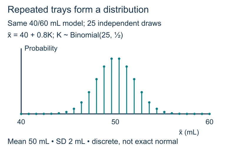 For 25 independent fills equally likely to be 40 or 60 mL, K is binomial with n = 25 and p = 0.5, and the tray mean is 40 + 0.8K. The exact distribution is discrete, centered at 50 mL with standard deviation 2 mL. A normal curve approximates its shape.
Reading a Normal Probability Plot
Common Mistakes to Avoid
Summary of Key Formulas
| Concept | Formula / Rule | When to Use |
|---|---|---|
| Z-score | \(z = \frac{X - \mu}{\sigma}\) | Convert to standard normal |
| Unstandardize | \(X = \mu + z\sigma\) | Inverse normal problems |
| Empirical Rule | 68 / 95 / 99.7 | Quick estimates within 1, 2, 3 SD |
| Left-tail \(P\) | \(P(Z \leq z)\) from table | "Less than" questions |
| Right-tail \(P\) | \(1 - P(Z \leq z)\) | "Greater than" questions |
| Between | \(P(z_1 \leq Z \leq z_2)\) | Subtract two cumulative areas |
Question 1 of 5
A distribution is \(N(80, 5)\). Using the Empirical Rule, approximately what percentage of values fall between 70 and 90?
Question 2 of 5
If \(X \sim N(200, 25)\) and \(X = 250\), what is the z-score?
Question 3 of 5
\(P(Z \leq 1.00) = 0.8413\). What is \(P(Z > 1.00)\)?
Question 4 of 5
A normal probability plot of a dataset shows points that curve sharply upward at the right end. This suggests the data are:
Question 5 of 5
Scores on a test are \(N(72, 8)\). A student wants to be in the top 5%. What is the minimum score needed? (Use \(z^* = 1.645\) for the 95th percentile.)