The Central
Limit Theorem
Discover why the normal distribution emerges from sampling: how \(\bar{X}\) behaves as \(n\) grows, regardless of the population shape.
What Is a Sampling Distribution?
Imagine you take a sample of size \(n\) from a population, compute the sample mean \(\bar{x}\), and repeat this thousands of times. The distribution of all those \(\bar{x}\) values is called the sampling distribution of the sample mean.
Population vs. Sampling Distribution
Why Does the CLT Matter?
In the real world, we rarely know the population distribution. The CLT gives us permission to use normal-based methods (z-scores, confidence intervals, hypothesis tests) even when the population is not normal.
The Central Limit Theorem: Formal Statement
From Skewed to Normal
A filling line that deposits one statistic for a whole tray
 A tray contains individual observations, but its average contributes one value to a distribution of sample means. Repeating the sampling process reveals how that statistic varies.
Build the distribution of tray means
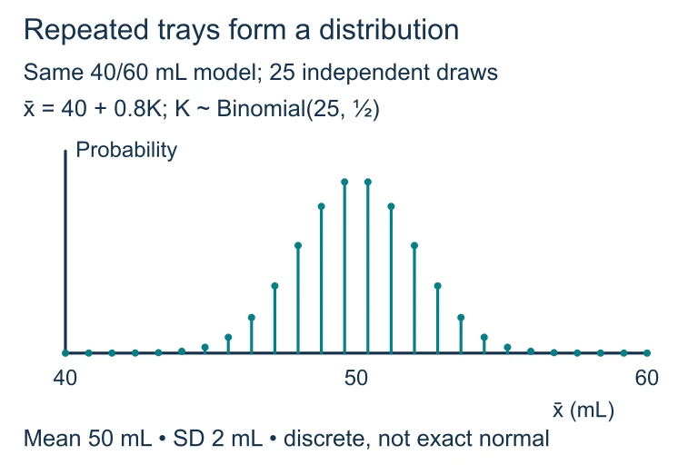 For 25 independent fills equally likely to be 40 or 60 mL, K is binomial with n = 25 and p = 0.5, and the tray mean is 40 + 0.8K. The exact distribution is discrete, centered at 50 mL with standard deviation 2 mL. A normal curve approximates its shape.
The Standard Error of \(\bar{X}\)
The standard deviation of the sampling distribution has a special name: the standard error. It measures how much \(\bar{x}\) typically varies from \(\mu\).
CLT vs. Law of Large Numbers
| Central Limit Theorem | Law of Large Numbers | |
|---|---|---|
| What it says | \(\bar{X}\) is approximately Normal for large \(n\) | \(\bar{X} \to \mu\) as \(n \to \infty\) |
| Focus | Shape of the distribution | Value of the average |
| Tells us about | Spread and symmetry of \(\bar{X}\) | Convergence of \(\bar{X}\) to \(\mu\) |
| Key use | Constructing z-scores, CIs | Justifying long-run frequencies |
Conditions for Applying the CLT
How to Apply the CLT
Example 1: Light Bulb Lifetimes
A factory produces light bulbs with a mean lifetime of \(\mu = 1200\) hours and standard deviation \(\sigma = 200\) hours. The distribution of lifetimes is right-skewed. If we take a random sample of \(n = 50\) bulbs, what is \(P(\bar{X} > 1240)\)?
Example 1: Visualized
Example 2: Commute Times
The mean commute time in a city is \(\mu = 35\) minutes with \(\sigma = 12\) minutes. A researcher samples \(n = 64\) commuters. Find the probability that the sample mean is between 33 and 37 minutes.
Example 3: Finding Sample Size
A quality inspector wants \(P(\bar{X}\) is within 5 units of \(\mu) \geq 0.95\). The population has \(\sigma = 20\). How large must \(n\) be?
Common Mistakes
Summary: CLT at a Glance
| Property | Individual Observation \(X\) | Sample Mean \(\bar{X}\) |
|---|---|---|
| Mean | \(\mu\) | \(\mu\) |
| Standard Deviation | \(\sigma\) | \(\sigma / \sqrt{n}\) |
| Shape | Same as population | Approximately Normal (large \(n\)) |
| Spread | Wider | Narrower (decreases with \(n\)) |
| Used for | Describing individuals | Inference about \(\mu\) |
Question 1 of 5
A population has \(\mu = 50\) and \(\sigma = 10\). For a random sample of size \(n = 25\), what is the standard error of \(\bar{X}\)?
Question 2 of 5
The Central Limit Theorem states that the sampling distribution of \(\bar{X}\) is approximately Normal when:
Question 3 of 5
A population is heavily right-skewed with \(\mu = 100\) and \(\sigma = 30\). A sample of \(n = 36\) is taken. What is \(P(\bar{X} < 95)\)?
Question 4 of 5
As sample size \(n\) increases, what happens to the standard error of \(\bar{X}\)?
Question 5 of 5
Which statement best describes the difference between the CLT and the Law of Large Numbers?