Summary Statistics
for a Quantitative Variable
Master the numbers that describe data: center, spread, and shape. Learn to calculate and interpret \(\bar{x}\), \(s\), \(Q_1\), \(Q_3\), and IQR.
What Are Summary Statistics?
Summary statistics are single numerical values that describe key features of a data set. Instead of listing every observation, we condense the data into numbers that capture its center, spread, and position.
Measures of Center
Visualizing Mean vs. Median
The Mean Formula
The sample mean is the sum of all observations divided by the number of observations:
Standard Deviation \(s\)
Standard deviation measures the average distance each observation falls from the mean. Larger \(s\) means more variability.
Quartiles and the IQR
Quartiles divide sorted data into four equal groups. The interquartile range measures the spread of the middle 50%.
Resistant vs. Non-Resistant Measures
A statistic is resistant if it is not strongly affected by outliers or extreme values. This distinction is critical when choosing which summary to report.
| Resistant | Non-Resistant | |
|---|---|---|
| Center | Median \(M\) | Mean \(\bar{x}\) |
| Spread | IQR | Standard deviation \(s\), Range |
| Best when | Skewed data or outliers present | Roughly symmetric, no outliers |
The Five-Number Summary
The five-number summary provides a complete positional picture of a distribution, and it is the basis for boxplots.
How to Compute Summary Statistics
Example 1: Finding the Median
A teacher records quiz scores for 9 students: 72, 85, 90, 65, 78, 92, 88, 70, 81. Find the median.
Example 2: Mean and Standard Deviation
Data: 4, 7, 8, 10, 11. Compute \(\bar{x}\) and \(s\).
Example 3: Five-Number Summary and Outliers
Data (sorted): 2, 5, 7, 8, 10, 12, 14, 15, 40. Find the five-number summary and check for outliers.
How Outliers Distort Statistics
Using the data from Example 3, compare the statistics with and without the outlier 40:
| Statistic | With 40 | Without 40 |
|---|---|---|
| Mean \(\bar{x}\) | 12.56 | 9.13 |
| Median \(M\) | 10 | 9 |
| Std. Dev. \(s\) | 11.10 | 4.49 |
| IQR | 8.5 | 7.0 |
Common Mistakes to Avoid
Summary of All Measures
| Measure | Formula / Method | Resistant? | Measures |
|---|---|---|---|
| Mean \(\bar{x}\) | \(\frac{\sum x_i}{n}\) | No | Center |
| Median \(M\) | Middle of sorted data | Yes | Center |
| Std. Dev. \(s\) | \(\sqrt{\frac{\sum(x_i - \bar{x})^2}{n-1}}\) | No | Spread |
| IQR | \(Q_3 - Q_1\) | Yes | Spread |
| Range | \(\text{Max} - \text{Min}\) | No | Spread |
Worked Example
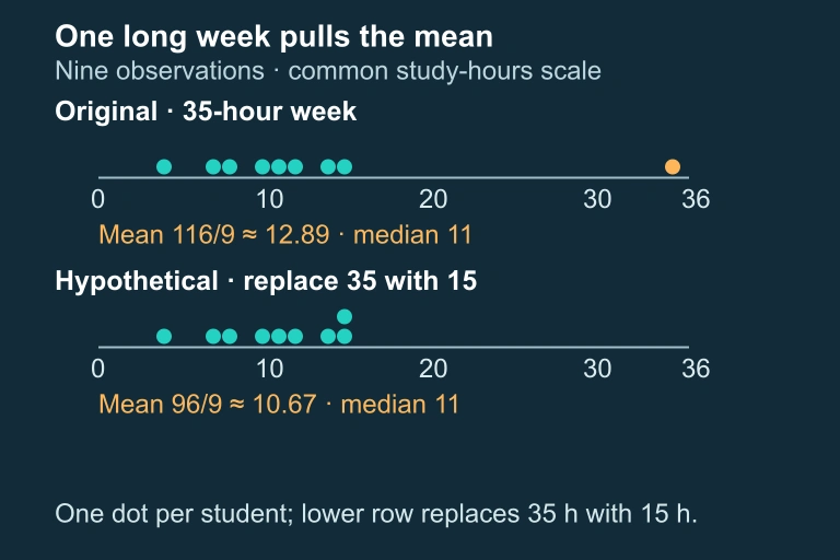
A researcher records the number of hours 9 college students spent studying during the week before a midterm exam: 4, 7, 8, 10, 11, 12, 14, 15, 35. Compute the mean, median, standard deviation, IQR, and identify any outliers using the 1.5 × IQR rule. Then explain which pair of summary statistics (mean/s or median/IQR) is more appropriate. Computing Summary Statistics for Study Hours Step 1 — Order the Data and Find n The data are already sorted: 4, 7, 8, 10, 11, 12, 14, 15, 35. Here n = 9. Step 2 — Compute the Mean x̄ = (4 + 7 + 8 + 10 + 11 + 12 + 14 + 15 + 35) / 9 = 116 / 9 ≈ 12.89 hours. x̄ ≈ 12.89 hours Step 3 — Find the Median With n = 9 observations, the median is the (9 + 1)/2 = 5th value in the ordered list. Counting: 4, 7, 8, 10, 11, 12, 14, 15, 35. Median = 11 hours Step 4 — Find Q₁ and Q₃ Lower half (below the median): 4, 7, 8, 10. Q₁ = median of lower half = (7 + 8)/2 = 7.5. Upper half (above the median): 12, 14, 15, 35. Q₃ = median of upper half = (14 + 15)/2 = 14.5. Q₁ = 7.5, Q₃ = 14.5, IQR = 7 Step 5 — Check for Outliers (1.5 × IQR Rule) Lower fence = Q₁ − 1.5 × IQR = 7.5 − 10.5 = −3. Upper fence = Q₃ + 1.5 × IQR = 14.5 + 10.5 = 25. The observation 35 exceeds the upper fence of 25, so it is flagged as an outlier. 35 is an outlier Step 6 — Compute the Standard Deviation Compute each squared deviation from x̄ ≈ 12.89: (4 − 12.89)² ≈ 79.03, (7 − 12.89)² ≈ 34.63, (8 − 12.89)² ≈ 23.88, (10 − 12.89)² ≈ 8.35, (11 − 12.89)² ≈ 3.56, (12 − 12.89)² ≈ 0.79, (14 − 12.89)² ≈ 1.23, (15 − 12.89)² ≈ 4.45, (35 − 12.89)² ≈ 488.85. Sum ≈ 644.77. s = √(644.77 / 8) = √80.60 ≈ 8.98. s ≈ 8.98 hours Step 7 — Choose the Appropriate Summary Because the distribution contains a high outlier (35 hours), it is right-skewed. The mean (12.89) is pulled above the median (11), and the standard deviation (8.98) is inflated by the outlier. The more appropriate summary uses the median and IQR: "The typical student studied about 11 hours, with the middle 50% studying between 7.5 and 14.5 hours (IQR = 7)."
Question 1 of 5
A data set has a strong right skew and several high outliers. Which pair of summary statistics best describes the center and spread?
Question 2 of 5
For the data set 3, 5, 7, 9, 11, what is the sample standard deviation \(s\)?
Question 3 of 5
A distribution is symmetric and bell-shaped. Which statement is true?
Question 4 of 5
For a data set, \(Q_1 = 20\) and \(Q_3 = 36\). Using the \(1.5 \times \text{IQR}\) rule, what is the upper fence for outliers?
Question 5 of 5
Why does the formula for sample standard deviation divide by \(n - 1\) instead of \(n\)?