01 / 20

Inference
Procedures

Master the art of selecting, implementing, and communicating the right statistical inference procedure for any scenario.

AP Statistics

What is Statistical Inference?

Statistical inference uses sample data to draw conclusions about a population parameter. The two main tools are confidence intervals (estimating a parameter) and significance tests (testing a claim about a parameter).

Confidence Interval
Estimates a range of plausible values for a parameter
Significance Test
Assesses evidence against a null hypothesis about a parameter

The Inference Decision Flowchart

What is the question? Estimate a parameter Test a claim Confidence Interval Significance Test 1 proportion 1 or 2 means 1 proportion 1 or 2 means

Parameters Drive the Procedure

The parameter you are investigating determines which formula, distribution, and conditions you use. Here are the core inference settings for AP Statistics:

One-sample \( z \)
For a single population proportion \( p \)
One-sample \( t \)
For a single population mean \( \mu \)
Two-sample \( z \)
For comparing two proportions \( p_1 - p_2 \)
Two-sample \( t \)
For comparing two means \( \mu_1 - \mu_2 \)

The Confidence Interval Formula

Every confidence interval in AP Statistics follows the same general structure:

Statistic
Point estimate from the sample: \( \hat{p} \) or \( \bar{x} \)
Critical Value
\( z^* \) for proportions, \( t^* \) for means: controls the confidence level
Standard Error
Measures variability of the statistic from sample to sample

The Significance Test Framework

Every hypothesis test follows a four-step process. AP readers look for all four steps explicitly stated:

1
State: Define hypotheses \( H_0 \) and \( H_a \), state the parameter and significance level \( \alpha \).
2
Plan: Name the procedure and check all conditions (Random, Normal, Independent).
3
Do: Compute the test statistic and the \( p \)-value.
4
Conclude: Compare \( p \)-value to \( \alpha \) and state your conclusion in context.

CI vs. Significance Test

Confidence Interval Significance Test
Purpose Estimate a parameter Test a claim about a parameter
Output Range of plausible values \( p \)-value and decision
Key formula part \(\text{stat} \pm z^*/t^* \cdot SE\) \(\dfrac{\text{stat} - \text{null}}{SE}\)
Standard error uses Sample statistic (\( \hat{p} \) or \( \bar{x} \)) Null value \( p_0 \) (for proportions)
Conclusion language "We are C% confident that..." "We do/do not reject \( H_0 \)..."

Conditions You Must Check

Before performing any inference procedure, verify these three conditions. Failure to check them loses points on the AP exam:

1
Random: Data come from a random sample or randomized experiment.
2
Normal (Large Counts / Large Sample): For proportions: \( np \geq 10 \) and \( n(1-p) \geq 10 \). For means: \( n \geq 30 \) or population is roughly normal.
3
Independent (10% Condition): Sample size is less than 10% of the population: \( n < 0.10N \). For experiments, groups are independent.

How to Apply the Procedure

1
Read the problem carefully. Identify the parameter: is it \( p \), \( \mu \), \( p_1 - p_2 \), or \( \mu_1 - \mu_2 \)?
2
Decide: estimate or test? "What proportion..." or "estimate the mean..." = CI. "Is there evidence that..." = test.
3
Name the procedure. e.g., "one-sample \( z \)-test for a proportion" or "two-sample \( t \)-interval for \( \mu_1 - \mu_2 \)".
4
Check conditions. Write out Random, Normal, Independent with specific numbers from the problem.
5
Calculate and conclude in context. Use the specific variable names and units from the problem.

Example 1: One-Sample \( z \)-Test

A company claims that 40% of its customers prefer Brand A. A random sample of 200 customers finds that 92 prefer Brand A. At \( \alpha = 0.05 \), is there evidence the true proportion differs from 0.40?

S
\( H_0: p = 0.40 \), \( H_a: p \neq 0.40 \), where \( p \) = true proportion preferring Brand A.
P
One-sample \( z \)-test for \( p \). Random: stated. Normal: \( 200(0.40) = 80 \geq 10 \), \( 200(0.60) = 120 \geq 10 \) ✓. Independent: \( 200 < 10\% \) of all customers ✓.
D
\( \hat{p} = 92/200 = 0.46 \). \( z = \dfrac{0.46 - 0.40}{\sqrt{0.40 \cdot 0.60 / 200}} = \dfrac{0.06}{0.03464} \approx 1.732 \). \( p\text{-value} = 2P(Z > 1.732) \approx 0.0832 \).
C
Since \( 0.0832 > 0.05 \), we fail to reject \( H_0 \). There is not convincing evidence that the true proportion differs from 0.40.

Example 2: One-Sample \( t \)-Interval

A random sample of 36 students has a mean study time of \( \bar{x} = 4.2 \) hours with \( s = 1.5 \) hours. Construct a 95% confidence interval for the true mean study time \( \mu \).

1
Procedure: One-sample \( t \)-interval for \( \mu \).
2
Conditions: Random ✓. Normal: \( n = 36 \geq 30 \) ✓ (CLT). Independent: \( 36 < 10\% \) of all students ✓.
3
Calculate: \( df = 35 \), \( t^* = 2.030 \). \( SE = 1.5 / \sqrt{36} = 0.25 \). Interval: \( 4.2 \pm 2.030(0.25) = (3.69, 4.71) \).
4
Interpret: We are 95% confident that the true mean study time for all students is between 3.69 and 4.71 hours.

Example 3: Two-Sample \( t \)-Test

Does a new teaching method improve scores? Group 1 (\( n_1 = 40 \), \( \bar{x}_1 = 78 \), \( s_1 = 10 \)) used the new method. Group 2 (\( n_2 = 35 \), \( \bar{x}_2 = 72 \), \( s_2 = 12 \)) used the traditional method. Test at \( \alpha = 0.05 \).

S
\( H_0: \mu_1 - \mu_2 = 0 \), \( H_a: \mu_1 - \mu_2 > 0 \). Parameter: difference in true mean scores.
P
Two-sample \( t \)-test. Random: randomized experiment ✓. Normal: both \( n \geq 30 \) ✓. Independent: groups are separate ✓.
D
\( SE = \sqrt{10^2/40 + 12^2/35} \approx 2.572 \). \( t = \dfrac{78 - 72}{2.572} \approx 2.333 \). With \( df \approx 65 \), \( p\text{-value} \approx 0.0114 \).
C
Since \( 0.0114 < 0.05 \), reject \( H_0 \). There is convincing evidence the new method produces higher mean scores.

Communicating Your Conclusion

How you write your conclusion matters as much as the calculation. AP readers grade your wording carefully. Here are the templates:

Common Mistakes to Avoid

✕ Wrong SE for Tests
Using \( \hat{p} \) instead of \( p_0 \) in the standard error for a one-proportion \( z \)-test.
✕ "Accept \( H_0 \)"
Never say "accept the null." Say "fail to reject \( H_0 \)": we cannot prove \( H_0 \) is true.
✕ No Context
Writing "reject \( H_0 \)" without stating what that means in terms of the original question.
✕ Skipping Conditions
Not checking Random, Normal, and Independent. You must show the work, not just say "conditions met."
✕ Using \( z \) for Means
When \( \sigma \) is unknown (almost always), use \( t \)-procedures for means, not \( z \).
✕ Misinterpreting CI
Saying "95% probability the parameter is in this interval." The parameter is fixed: it either is or isn't in the interval.

Procedure Summary Table

Procedure Parameter Test Statistic SE Formula
1-prop \( z \) \( p \) \( z = \dfrac{\hat{p} - p_0}{SE} \) \( \sqrt{\dfrac{p_0(1-p_0)}{n}} \)
1-sample \( t \) \( \mu \) \( t = \dfrac{\bar{x} - \mu_0}{SE} \) \( \dfrac{s}{\sqrt{n}} \)
2-prop \( z \) \( p_1 - p_2 \) \( z = \dfrac{\hat{p}_1 - \hat{p}_2}{SE} \) \( \sqrt{\hat{p}_c(1-\hat{p}_c)\left(\frac{1}{n_1}+\frac{1}{n_2}\right)} \)
2-sample \( t \) \( \mu_1 - \mu_2 \) \( t = \dfrac{\bar{x}_1 - \bar{x}_2}{SE} \) \( \sqrt{\dfrac{s_1^2}{n_1} + \dfrac{s_2^2}{n_2}} \)

Worked Example: Full Inference Write-Up

A researcher wants to determine whether students have a nonzero mean score difference after a new tutoring program on a standardized math assessment. A random sample of 20 students is selected, and each student takes the assessment before and after completing the eight-week program. The mean of the differences (after − before) is x̄_(d) = 4.8 points, and the standard deviation of the differences is s_(d) = 7.2 points. A dotplot of the differences shows a roughly symmetric distribution with no outliers. Test at the α = 0.05 significance level whether the population mean after-minus-before difference is nonzero. Paired t-Test: Tutoring Program Step 1 — Name the Procedure & Define the Parameter We will perform a paired t-test because the same 20 students are measured before and after the program, creating a natural pairing. Let μ_(d) = the true mean difference in assessment scores (after − before) for all students who could complete this tutoring program. Procedure: Paired t-test for μ_d Step 2 — State Hypotheses H₀: μ_(d) = 0 (the population mean after-minus-before difference is zero). Hₐ: μ_(d) ≠ 0 (the population mean after-minus-before difference is nonzero). Use a two-sided alternative because either direction of change is relevant. H₀: μ_d = 0; Hₐ: μ_d ≠ 0 Step 3 — Check Conditions Random: The problem states that a random sample of 20 students was selected. ✓ Independence: We can reasonably assume that 20 students are less than 10% of all students who could potentially complete the program, so the differences are approximately independent. ✓ Normal: The sample size is n = 20 (less than 30), but the dotplot of differences shows a roughly symmetric distribution with no outliers, so it is reasonable to assume the population of differences is approximately normal. ✓ All three conditions met Step 4 — Calculate the Test Statistic and p-Value t = (x̄_(d) − 0) / (s_(d) / √n) = (4.8 − 0) / (7.2 / √20) = 4.8 / 1.6099 ≈ 2.981. With df = 20 − 1 = 19 and a two-sided test, the p-value = 2 × P(t > 2.981) ≈ 0.0077 (using calculator: T-Test or tcdf). t ≈ 2.981, df = 19, p-value ≈ 0.0077 Step 5 — State the Conclusion in Context Because the p-value (about 0.0077) is below α = 0.05, reject H₀. There is convincing evidence that the mean after-minus-before score difference in the population represented by the sample is not zero. This uncontrolled before/after design does not by itself establish that the tutoring program caused the change. Reject H₀: evidence of a nonzero mean difference, not proof of program causation. THE 4-PART TEMPLATE Every hypothesis test on the AP exam should follow the same four-part structure: (1) State — name the procedure, define parameters, write hypotheses; (2) Plan — check conditions with evidence from the problem; (3) Do — compute the test statistic and p-value; (4) Conclude — make a decision and interpret in context. Think of it like a lab report in science: the structure is non-negotiable, and skipping a section means incomplete work.
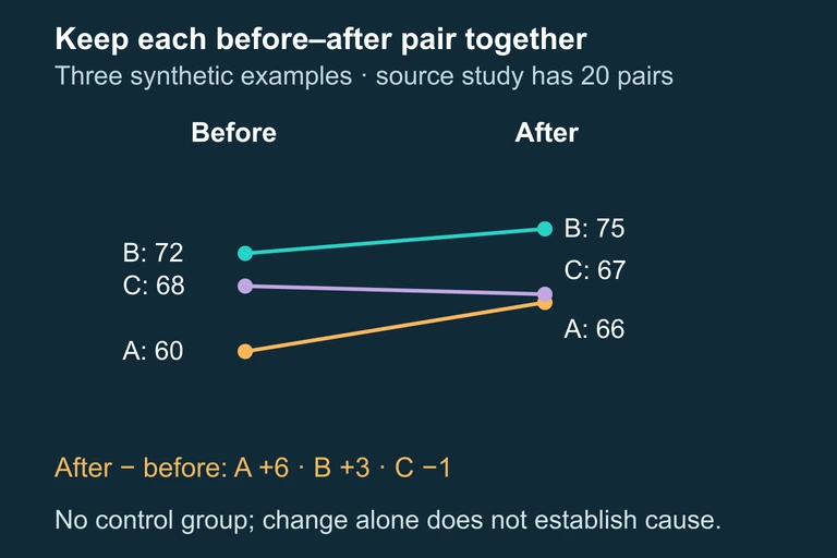
Three explicitly synthetic paired records: A changes 60 to 66, B 72 to 75 and C 68 to 67. Differences are +6,+3,−1; these do not supply the source study’s twenty-person summary.
Each student’s after score stays linked to that student’s before score; the individual pairs are illustrative. The summary covers 20 students.

Question 1 of 5

A researcher wants to estimate the proportion of adults who support a new policy. She surveys a random sample of 500 adults. Which inference procedure should she use?

Question 2 of 5

When performing a one-proportion \( z \)-test, which value should be used to compute the standard error?

Question 3 of 5

A 95% confidence interval for \( \mu \) is \( (12.3, 15.7) \). Which interpretation is correct?

Question 4 of 5

A test yields a \( p \)-value of 0.03. The significance level is \( \alpha = 0.05 \). Which conclusion is appropriate?

Question 5 of 5

A scientist compares the mean reaction times of two independent groups (\( n_1 = 25 \), \( n_2 = 30 \)). Population standard deviations are unknown. Which procedure is appropriate?