Sampling Distributions
Differences in Sample Means
Explore how the distribution of \(\bar{X}_1 - \bar{X}_2\) behaves, what determines its center and spread, and how to use it for inference about two populations.
Why Compare Two Means?
In statistics, we often want to compare two populations. For example: Is the average blood pressure lower for a treatment group than a control group? Does one fertilizer produce a higher mean yield than another?
The natural estimator for the difference in population means \(\mu_1 - \mu_2\) is the difference in sample means \(\bar{X}_1 - \bar{X}_2\). But a single sample gives only one value: to draw conclusions, we need to understand the entire sampling distribution of that difference.
Visualizing the Sampling Distribution
Three Building Blocks
Core Formulas
Why Variances Add
For independent random variables, variances always add: whether the operation is addition or subtraction. The property \(\text{Var}(A - B) = \text{Var}(A) + \text{Var}(B)\) holds because independence eliminates the covariance term.
Shape: The CLT Condition
The Central Limit Theorem guarantees that \(\bar{X}_1 - \bar{X}_2\) is approximately Normal when:
One Mean vs. Difference of Means
| One Sample Mean \(\bar{X}\) | Difference \(\bar{X}_1 - \bar{X}_2\) | |
|---|---|---|
| Center | \(\mu\) | \(\mu_1 - \mu_2\) |
| Std Dev | \(\dfrac{\sigma}{\sqrt{n}}\) | \(\sqrt{\dfrac{\sigma_1^2}{n_1} + \dfrac{\sigma_2^2}{n_2}}\) |
| Shape | Normal if population Normal or \(n \geq 30\) | Normal if both populations Normal or both \(n \geq 30\) |
| Parameters | \(\mu, \sigma, n\) | \(\mu_1, \mu_2, \sigma_1, \sigma_2, n_1, n_2\) |
Step-by-Step Application
Example 1: Finding the Standard Deviation
A researcher studies test scores in two schools. School A: \(\mu_1 = 78\), \(\sigma_1 = 10\), \(n_1 = 40\). School B: \(\mu_2 = 72\), \(\sigma_2 = 12\), \(n_2 = 50\). Find the mean and standard deviation of \(\bar{X}_1 - \bar{X}_2\).
Example 2: Finding a Probability
Using the same schools (\(\mu_{\bar{X}_1-\bar{X}_2}=6\), \(\sigma=2.32\)): What is the probability that \(\bar{X}_1 - \bar{X}_2 < 2\)?
There is only about a 4.3% chance that the difference in sample means falls below 2, given the true difference is 6.
Example 3: Effect of Sample Size
What happens to the standard deviation if we increase both sample sizes to \(n_1 = 100\) and \(n_2 = 100\), keeping \(\sigma_1 = 10\) and \(\sigma_2 = 12\)?
SD \(\approx 2.32\)
SD \(\approx 1.56\)
The 10% Condition
When sampling without replacement, observations are not truly independent. The standard deviation formula works well only if each sample is small relative to its population:
The Complete Picture
Common Mistakes
A listening study with fixed response cards and moving treatment badges
 Measurements taken from the same person remain linked. Compare within-person differences instead of treating the two columns as independent samples.
Keep the pairs linked
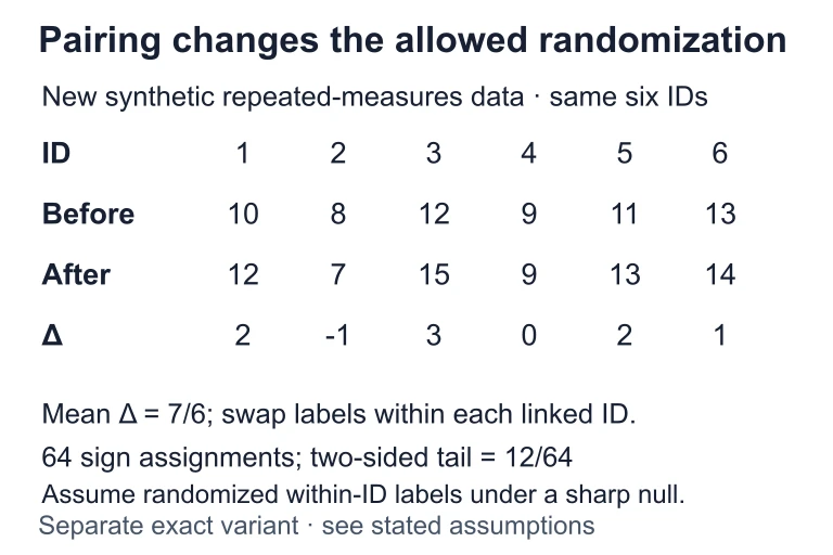 Suppose the same six IDs have differences 2, −1, 3, 0, 2 and 1, averaging 7/6. Under a sharp zero-effect null with randomized or exchangeable within-ID labels, 2⁶ = 64 sign assignments are allowed; 12 have absolute mean at least 7/6. Repeated measurement alone does not establish that exchangeability.
Summary: Key Facts
| Property | Formula / Rule |
|---|---|
| Mean | \(\mu_1 - \mu_2\) |
| Standard Deviation | \(\sqrt{\dfrac{\sigma_1^2}{n_1} + \dfrac{\sigma_2^2}{n_2}}\) |
| Shape | Normal (if both pops Normal or both \(n \geq 30\)) |
| Independence | Two samples must be independent |
| 10% Condition | \(n_1 \leq 0.10 N_1\) and \(n_2 \leq 0.10 N_2\) |
| Effect of larger \(n\) | SD decreases, distribution narrows |
Question 1 of 5
The mean of the sampling distribution of \(\bar{X}_1 - \bar{X}_2\) equals:
Question 2 of 5
When computing the standard deviation of \(\bar{X}_1 - \bar{X}_2\), why do the variance terms add rather than subtract?
Question 3 of 5
Population 1 has \(\mu_1 = 50, \sigma_1 = 8, n_1 = 64\). Population 2 has \(\mu_2 = 45, \sigma_2 = 6, n_2 = 36\). Find \(\sigma_{\bar{X}_1 - \bar{X}_2}\).
Question 4 of 5
Which of the following is NOT a required condition for the sampling distribution of \(\bar{X}_1 - \bar{X}_2\) to be approximately Normal?
Question 5 of 5
If you quadruple both sample sizes (multiply each by 4), the standard deviation of \(\bar{X}_1 - \bar{X}_2\) is multiplied by: