Sampling Distributions
for Sample Proportions
Understand how sample proportions behave across repeated samples, and learn to compute the mean and standard deviation of \(\hat{p}\).
What Is a Sample Proportion?
When we take a random sample of size \(n\) from a population and count the number of "successes," the sample proportion is:
\(\hat{p}\) is a statistic: it varies from sample to sample. The true population proportion \(p\) is a fixed parameter we are trying to estimate.
Why Does \(\hat{p}\) Vary?
Imagine a population where 60% favor a policy (\(p = 0.60\)). If you draw many random samples of \(n = 100\), each sample will yield a different \(\hat{p}\).
Visualizing the Sampling Distribution
If we repeated the sampling process thousands of times and plotted all \(\hat{p}\) values, we would see a bell-shaped curve centered at the true proportion \(p\).
Mean and Standard Deviation of \(\hat{p}\)
The sampling distribution of \(\hat{p}\) has two key parameters:
Conditions for Normal Approximation
The sampling distribution of \(\hat{p}\) is approximately normal only when certain conditions are met:
The Normal Model for \(\hat{p}\)
This means we can use z-scores to find probabilities about \(\hat{p}\):
This z-score tells us how many standard deviations a particular \(\hat{p}\) is from the true proportion \(p\).
Parameter vs. Statistic
A critical distinction in inference: do not confuse the population parameter with the sample statistic.
| Parameter \(p\) | Statistic \(\hat{p}\) | |
|---|---|---|
| What is it? | True population proportion | Sample proportion |
| Fixed or varies? | Fixed (one value) | Varies (sample to sample) |
| Known? | Usually unknown | Computed from data |
| Notation | \(p\) | \(\hat{p}\) |
| Has a distribution? | No (it is a constant) | Yes: the sampling distribution |
Effect of Sample Size on Spread
As the sample size \(n\) increases, the standard deviation \(\sigma_{\hat{p}}\) decreases, and the distribution becomes more concentrated around \(p\).
How to Apply the Sampling Distribution
Example 1: Checking Conditions
A city has 50,000 voters, and 40% support a new park. A pollster takes an SRS of \(n = 200\). Can we use the normal model for \(\hat{p}\)?
Example 2: Finding a Probability
Continuing the previous example: what is the probability that \(\hat{p}\) exceeds 0.45?
Example 3: Between Two Values
A factory produces light bulbs with a 5% defect rate (\(p = 0.05\)). In a random sample of \(n = 500\), what is \(P(0.03 < \hat{p} < 0.07)\)?
When Conditions Fail
If the large counts condition is not met, the sampling distribution is skewed, not normal. The normal approximation gives inaccurate probabilities.
Common Mistakes to Avoid
Summary of Key Formulas
| Property | Formula / Rule |
|---|---|
| Mean of \(\hat{p}\) | \(\mu_{\hat{p}} = p\) |
| SD of \(\hat{p}\) | \(\sigma_{\hat{p}} = \sqrt{\frac{p(1-p)}{n}}\) |
| Shape | Approximately normal (if conditions met) |
| Large Counts | \(np \geq 10\) and \(n(1-p) \geq 10\) |
| Independence | \(n \leq 0.10N\) (10% condition) |
| Z-score | \(z = \frac{\hat{p} - p}{\sigma_{\hat{p}}}\) |
Visual Explanation: From Population to Sampling Distribution
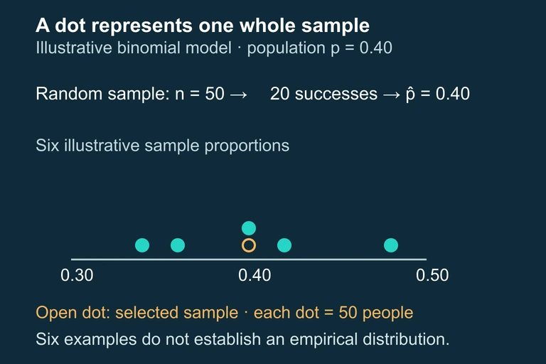
The following diagram illustrates the conceptual process of constructing a sampling distribution. Imagine a large population with true proportion p = 0.40. We repeatedly draw random samples of size n = 50, compute p̂ for each sample, and then plot the distribution of all those p̂ values. The resulting histogram forms the sampling distribution, which—when the Large Counts Condition is satisfied—takes on the characteristic bell shape of a normal distribution centered at p. The diagram traces the process from a population with p = 0.40, through repeated sampling at n = 50, to the resulting bell-shaped sampling distribution of p̂. The dashed pink line marks the center at p = 0.40, while the amber dashed lines indicate ±1 standard deviation (σ_(p̂) ≈ 0.069). Notice several important features in the diagram. First, each individual sample produces a different p̂ value—0.38, 0.44, 0.36, and so on—reflecting natural sampling variability. Second, when we aggregate thousands of these p̂ values, the histogram forms a smooth, symmetric bell curve centered on the true population proportion p = 0.40. Third, the spread of this distribution—governed by σ_(p̂) = √(0.40 × 0.60 / 50) ≈ 0.069—quantifies how much p̂ typically deviates from p in a single sample. About 68% of all sample proportions fall within one standard deviation of the center, and about 95% fall within two standard deviations.
Question 1 of 5
If \(p = 0.30\) and \(n = 200\), what is the standard deviation of the sampling distribution of \(\hat{p}\)?
Question 2 of 5
A population has \(p = 0.10\) and we sample \(n = 50\). Can we use the normal approximation for \(\hat{p}\)?
Question 3 of 5
If you quadruple the sample size from \(n\) to \(4n\), the standard deviation of \(\hat{p}\) is:
Question 4 of 5
For the sampling distribution of \(\hat{p}\), which statement is true?
Question 5 of 5
In a large population, 72% own a smartphone. In a random sample of \(n = 150\), what is the approximate probability that \(\hat{p} < 0.68\)?