Sampling Distributions
for Sample Means
Discover how sample means behave when drawn repeatedly from a population, and why the Central Limit Theorem is the most powerful idea in statistics.
What Is a Sampling Distribution?
Imagine you take a random sample of size \( n \) from a population and compute the sample mean \( \bar{x} \). Now repeat that process thousands of times. The distribution of all those \( \bar{x} \) values is called the sampling distribution of the sample mean.
Population vs. Sampling Distribution
Why Does This Matter?
Mean and Standard Deviation of \( \bar{x} \)
If the population has mean \( \mu \) and standard deviation \( \sigma \), then the sampling distribution of \( \bar{x} \) for samples of size \( n \) has:
A filling line that deposits one statistic for a whole tray
 A tray contains individual observations, but its average contributes one value to a distribution of sample means. Repeating the sampling process reveals how that statistic varies.
Build the distribution of tray means
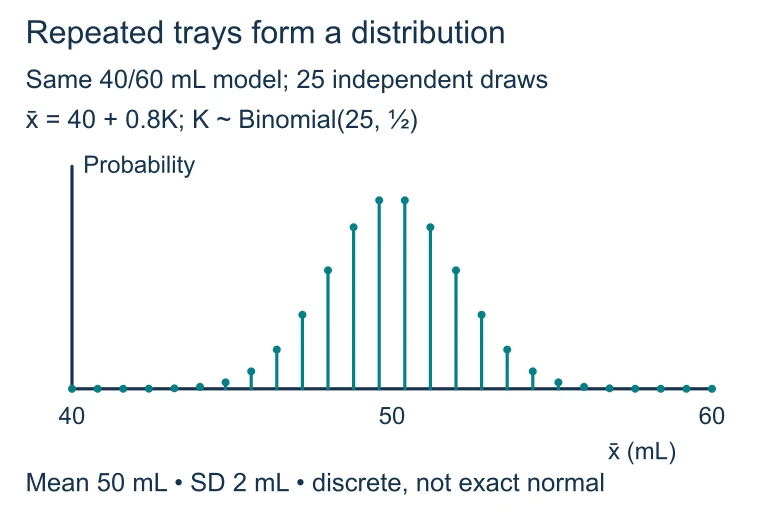 For 25 independent fills equally likely to be 40 or 60 mL, K is binomial with n = 25 and p = 0.5, and the tray mean is 40 + 0.8K. The exact distribution is discrete, centered at 50 mL with standard deviation 2 mL. A normal curve approximates its shape.
The Central Limit Theorem
Visualizing the CLT as \( n \) Grows
When Is \( n \) Large Enough?
\( \sigma \) vs. \( \sigma_{\bar{x}} \): A Key Distinction
| Population SD: \( \sigma \) | Standard Error: \( \sigma_{\bar{x}} \) | |
|---|---|---|
| Measures | Spread of individual values | Spread of sample means |
| Formula | \( \sigma \) | \( \frac{\sigma}{\sqrt{n}} \) |
| Effect of \( n \) | Does not change | Decreases as \( n \) increases |
| Interpretation | How far a single observation is from \( \mu \) | How far a sample mean is from \( \mu \) |
The 10% Condition
The formula \( \sigma_{\bar{x}} = \frac{\sigma}{\sqrt{n}} \) assumes samples are drawn with replacement or from an infinite population. In practice, we sample without replacement, which slightly reduces variability.
If the sample is more than 10% of the population, use the finite population correction factor: \( \sigma_{\bar{x}} = \frac{\sigma}{\sqrt{n}} \cdot \sqrt{\frac{N - n}{N - 1}} \). On the AP exam, the 10% condition is usually satisfied.
How to Apply the Sampling Distribution
Example 1: Battery Life
A factory produces batteries with a mean life of \( \mu = 500 \) hours and standard deviation \( \sigma = 40 \) hours. A quality inspector tests a random sample of \( n = 64 \) batteries. What is the probability that the sample mean life is less than 490 hours?
Example 1: Visual
Example 2: Test Scores
SAT Math scores are normally distributed with \( \mu = 528 \) and \( \sigma = 117 \). A school counselor randomly selects \( n = 36 \) students. Find the probability that the sample mean exceeds 550.
Example 3: Between Two Values
The weight of cereal boxes has \( \mu = 368 \) g and \( \sigma = 15 \) g. For a sample of \( n = 25 \) boxes, find \( P(365 < \bar{x} < 372) \).
Common Mistakes to Avoid
Summary: Key Facts at a Glance
| Property | Formula / Rule |
|---|---|
| Mean of \( \bar{x} \) | \( \mu_{\bar{x}} = \mu \) |
| Standard Error | \( \sigma_{\bar{x}} = \frac{\sigma}{\sqrt{n}} \) |
| Shape (CLT) | Approximately \( N\!\left(\mu, \frac{\sigma}{\sqrt{n}}\right) \) for large \( n \) |
| z-score | \( z = \frac{\bar{x} - \mu}{\sigma / \sqrt{n}} \) |
| Normal population | \( \bar{x} \) is exactly normal for any \( n \) |
| Rule of thumb | \( n \geq 30 \) for non-normal populations |
| 10% Condition | \( n \leq 0.10 \times N \) |
Question 1 of 5
A population has \( \mu = 80 \) and \( \sigma = 20 \). For a random sample of \( n = 100 \), what is the standard error of \( \bar{x} \)?
Question 2 of 5
Which of the following increases as the sample size \( n \) increases?
Question 3 of 5
Heights in a city are normally distributed with \( \mu = 170 \) cm and \( \sigma = 8 \) cm. For a sample of \( n = 16 \), find \( P(\bar{x} > 174) \).
Question 4 of 5
A population distribution is strongly right-skewed. A researcher takes a sample of \( n = 10 \). Which statement is most accurate?
Question 5 of 5
A machine fills bottles with a mean of \( \mu = 500 \) mL and \( \sigma = 12 \) mL. A quality team samples \( n = 36 \) bottles. What is the probability that the sample mean is between 497 and 503 mL?