01 / 20

Random Variables &
Probability Distributions

Learn how to assign numerical values to random outcomes, build probability distributions, and compute expected value and standard deviation.

AP Statistics

What Is a Random Variable?

A random variable is a function that assigns a numerical value to each outcome in a sample space. We denote random variables with capital letters like \(X\), \(Y\), or \(Z\).

The key idea: we move from describing outcomes in words to describing them with numbers, which lets us do calculations.

Discrete vs Continuous Random Variables

Discrete
Takes on a countable number of values. You can list them out: \(0, 1, 2, 3, \ldots\)
Continuous
Takes on any value in an interval. You cannot list them: heights, weights, times.

Why Probability Distributions Matter

A probability distribution tells us the complete story of a random variable: every value it can take and how likely each value is. This unlocks powerful tools.

1
Predict outcomes. What is the most likely result of an experiment?
2
Measure center. Compute the expected value: the long-run average.
3
Measure spread. Compute the standard deviation: how variable are results?
4
Make decisions. Is a gamble worth it? Should a company insure against a risk?

Building a Probability Distribution

For a discrete random variable, we list every value \(x_i\) alongside its probability \(P(X = x_i)\). Two rules must hold:

Rule 1
Every probability is between 0 and 1: \(0 \leq P(X = x_i) \leq 1\)
Rule 2
All probabilities sum to 1: \(\sum P(X = x_i) = 1\)

Visualizing with a Probability Histogram

Let \(X\) = number of heads in 3 coin flips. The distribution and histogram:

0 0.125 0.25 0.375 0 1 2 3 1/8 3/8 3/8 1/8 Number of Heads (X) P(X)

The Expected Value \(\mu_X\)

The expected value (or mean) of a discrete random variable is the long-run average: what you would get on average if you repeated the experiment forever.

The expected value does not have to be a value \(X\) can actually take. It is a weighted average, not a prediction of a single trial.

Variance and Standard Deviation

The variance measures how spread out the distribution is, and the standard deviation is its square root.

Each squared deviation \((x_i - \mu_X)^2\) is weighted by how likely that value is. Larger spread means larger \(\sigma_X\).

\(\mu_X\) vs \(\bar{x}\): A Key Distinction

\(\mu_X\) (Expected Value) \(\bar{x}\) (Sample Mean)
What is it? Theoretical long-run average Average of observed data
Source Probability distribution Collected sample
Changes? Fixed (parameter) Varies sample to sample
Notation \(\mu_X = E(X)\) \(\bar{x} = \frac{\sum x_i}{n}\)

How to Analyze a Distribution

1
List all values. Identify every possible value \(x_i\) the random variable can take.
2
Assign probabilities. Determine \(P(X = x_i)\) for each value. Verify they sum to 1.
3
Compute \(\mu_X\). Multiply each \(x_i \cdot P(X = x_i)\) and sum.
4
Compute \(\sigma_X^2\). Find each \((x_i - \mu_X)^2 \cdot P(X = x_i)\) and sum.
5
Compute \(\sigma_X\). Take the square root of the variance.

Worked Example: Raffle Ticket

A raffle has 100 tickets. One winner gets \$50, one gets \$20, and 98 get \$0. Each ticket costs \$1. Let \(X\) = net profit.

\(x_i\) \$49 \$19 -\$1
\(P(X = x_i)\) 1/100 1/100 98/100

Worked Example: Standard Deviation

Using the raffle from the previous slide with \(\mu_X = -0.30\), find \(\sigma_X\).

Example: Interpreting a Distribution Graph

A random variable \(X\) represents the number of defective items in a batch of 4. The distribution is shown below.

0 0.1 0.2 0.3 0.4 0 1 2 3 4 0.41 0.37 0.16 0.05 0.01 Number of Defects (X)

Common Mistakes to Avoid

✕ Probabilities don't sum to 1
Always verify \(\sum P(X = x_i) = 1\). A missing value makes the entire table invalid.
✕ Forgetting to square deviations
Variance uses \((x_i - \mu_X)^2\), not \(|x_i - \mu_X|\). Squaring prevents cancellation of positive and negative.
✕ Confusing \(\mu_X\) with mode
The expected value is a weighted average, not the most common outcome. \(\mu_X\) may not even be a possible value of \(X\).

Summary of Key Formulas

Concept Formula Interpretation
Expected Value \(\mu_X = \sum x_i \cdot P(X=x_i)\) Long-run average
Variance \(\sigma_X^2 = \sum (x_i - \mu_X)^2 \cdot P(X=x_i)\) Average squared spread
Std Deviation \(\sigma_X = \sqrt{\sigma_X^2}\) Typical distance from \(\mu_X\)
Validity Check \(\sum P(X=x_i) = 1\), all \(P(X=x_i) \geq 0\) Must hold for any distribution

Worked Example: Expected Value and Standard Deviation

A small insurance company offers a one-year policy that pays $10,000 for a major claim, $2,000 for a minor claim, and $0 if no claim is filed. Historical data show that the probability of a major claim is 0.02, the probability of a minor claim is 0.08, and the probability of no claim is 0.90. The company charges a premium of $500 per policy. Let X represent the profit the company earns on a randomly selected policy. Find the expected value and standard deviation of X. Computing E(X) and σ_X for an Insurance Profit Model Step 1 — Define the Random Variable and Build the Distribution Table Profit = Premium − Payout. If no claim: X = 500 − 0 = 500. If minor claim: X = 500 − 2000 = −1500. If major claim: X = 500 − 10000 = −9500. The distribution is: P(X = 500) = 0.90, P(X = −1500) = 0.08, P(X = −9500) = 0.02. Verify: 0.90 + 0.08 + 0.02 = 1.00 ✓ Three possible profit values: 500, −1500, −9500 Step 2 — Compute the Expected Value E(X) E(X) = Σ xᵢ · P(X = xᵢ) = (500)(0.90) + (−1500)(0.08) + (−9500)(0.02) = 450 + (−120) + (−190) = 140. The expected profit is $140 per policy. E(X) = $140 Step 3 — Compute the Variance Var(X) Var(X) = Σ (xᵢ − μ)² · P(X = xᵢ). For x = 500: (500 − 140)² × 0.90 = (360)² × 0.90 = 129,600 × 0.90 = 116,640. For x = −1500: (−1500 − 140)² × 0.08 = (−1640)² × 0.08 = 2,689,600 × 0.08 = 215,168. For x = −9500: (−9500 − 140)² × 0.02 = (−9640)² × 0.02 = 92,929,600 × 0.02 = 1,858,592. Var(X) = 116,640 + 215,168 + 1,858,592 = 2,190,400. Var(X) = 2,190,400 Step 4 — Compute the Standard Deviation σ_X σ_X = √(Var(X)) = √(2,190,400) ≈ 1,480.07. Interpretation: On average, the company's profit per policy deviates from the mean of $140 by approximately $1,480. This high standard deviation relative to the mean indicates substantial variability — a major claim, though rare, generates a large loss that drives up the spread. σ_X ≈ $1,480.07 $500 premium, three-outcome distribution. Interpretation Matters On the AP exam, you will lose credit if you only compute a number without interpreting it in context. Always state the meaning: "The company expects to earn an average profit of $140 per policy in the long run" is much stronger than simply writing "μ = 140." Likewise, describe what the standard deviation tells you about the variability of the random variable.
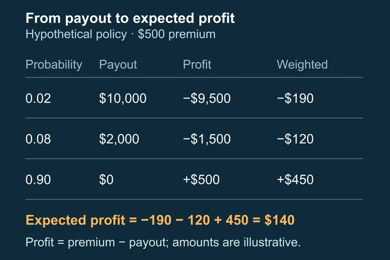
A $500-premium, three-outcome insurance distribution: profits −9500,−1500,500 with probabilities 0.02,0.08,0.90 and expected profit 140.
Company profit is premium minus payout, and expected profit weights each mutually exclusive modeled outcome by its probability.

Question 1 of 5

A random variable \(X\) has the distribution: \(P(X=1)=0.3\), \(P(X=2)=0.5\), \(P(X=3)=0.2\). What is \(E(X)\)?

Question 2 of 5

Which of the following is not a valid probability distribution?

Question 3 of 5

A game costs \$5 to play. You win \$20 with probability \(0.2\) and \$0 otherwise. What is your expected net profit?

Question 4 of 5

If \(X\) counts the number of heads in 2 fair coin flips, what is \(\text{Var}(X)\)?

Question 5 of 5

The expected value of a random variable \(X\) is \(\mu_X = 3.7\). Which statement is true?