01 / 21

Mean & Standard
Deviation

Master the expected value and spread of random variables: the building blocks of probability and inference in statistics.

AP Statistics

What Is a Random Variable?

A random variable assigns a numerical value to each outcome of a random process. We use uppercase letters like \(X\) to name them, and lowercase \(x\) for specific values they can take.

Discrete
Countable set of outcomes: number of heads in 5 flips, roll of a die
Continuous
Any value in an interval: height, temperature, time to finish a race

Probability Distribution Table

A discrete random variable is fully described by listing every possible value alongside its probability. The probabilities must sum to 1.

\(x\) 0 1 2 3
\(P(X = x)\) 0.10 0.30 0.40 0.20

Visualizing the Distribution

0 0.10 0.20 0.30 0.40 0 1 2 3 0.10 0.30 0.40 0.20
\(\text{mean} = 1.7\)
x
\(P(X=x)\)

The Mean (Expected Value)

The mean of a discrete random variable \(X\) is the weighted average of all possible values, weighted by their probabilities. We write it as \(\mu_X\) or \(E(X)\).

This is not the same as a simple average of the values. Each value is weighted by how likely it is to occur. The mean represents the long-run average if the experiment is repeated many times.

Variance and Standard Deviation

The variance measures how far the values spread from the mean, on average. The standard deviation is simply the square root, returning us to the original units.

A larger \(\sigma_X\) means outcomes are more spread out from the mean. A \(\sigma_X\) of zero means the variable always takes the same value.

Mean vs. Standard Deviation

Mean \(\mu_X\)
Where the distribution is centered: the long-run average value
SD \(\sigma_X\)
How much the distribution is spread out: the typical distance from the mean
Small SD Large SD same mean same mean

Linear Transformations: \(Y = a + bX\)

If you transform every value of \(X\) by adding a constant \(a\) and multiplying by a constant \(b\), the mean and standard deviation change in predictable ways.

Combining Independent Variables

When \(X\) and \(Y\) are independent random variables, we can find the mean and variance of their sum or difference.

How to Calculate Step by Step

1
List all values and probabilities. Write the full probability distribution table for \(X\).
2
Compute the mean. Multiply each \(x_i\) by its \(P(x_i)\) and sum: \(\mu_X = \sum x_i \cdot P(x_i)\).
3
Find each squared deviation. Calculate \((x_i - \mu_X)^2\) for every value.
4
Compute the variance. Multiply each squared deviation by its probability and sum: \(\sigma_X^2 = \sum (x_i - \mu_X)^2 \cdot P(x_i)\).
5
Take the square root to get the standard deviation: \(\sigma_X = \sqrt{\sigma_X^2}\).

Example 1: Finding \(\mu_X\)

A spinner lands on the values 1, 2, 3, or 4 with the probabilities shown. Find the mean \(\mu_X\).

\(x\) 1 2 3 4
\(P(X = x)\) 0.15 0.25 0.35 0.25

Example 2: Finding \(\sigma_X\)

Using the same spinner from Example 1 with \(\mu_X = 2.70\), find the standard deviation \(\sigma_X\).

\(x_i\) \((x_i - 2.70)^2\) \(\times P(x_i)\)
12.890.4335
20.490.1225
30.090.0315
41.690.4225

Example 3: Linear Transform

A game charges \(\$2\) to play the spinner from Example 1 and pays \(\$3\) for each point. Your profit is \(Y = 3X - 2\). Find \(\mu_Y\) and \(\sigma_Y\).

The expected profit per game is \(\$6.10\) with a standard deviation of \(\$3.015\).

Example 4: Combining Two Variables

Juan's daily commute time by bus has \(\mu_X = 25\) min and \(\sigma_X = 4\) min. His walk from the bus stop has \(\mu_Y = 8\) min and \(\sigma_Y = 2\) min. If \(X\) and \(Y\) are independent, find the mean and standard deviation of his total commute \(T = X + Y\).

Common Mistakes

✕ Adding SDs directly
When combining variables, add variances (\(\sigma^2\)), then take the square root. Never add standard deviations.
✕ Subtracting variances
For \(X - Y\), the variance is \(\sigma_X^2 + \sigma_Y^2\), not \(\sigma_X^2 - \sigma_Y^2\). Variances always add.
✕ Simple average for mean
The mean is a weighted average. Don't compute \((x_1 + x_2 + \ldots)/n\) unless all probabilities are equal.

Summary of Key Formulas

Operation Mean Variance
Definition \(\sum x_i P(x_i)\) \(\sum (x_i - \mu)^2 P(x_i)\)
\(Y = a + bX\) \(a + b\mu_X\) \(b^2 \sigma_X^2\)
\(X + Y\) (indep.) \(\mu_X + \mu_Y\) \(\sigma_X^2 + \sigma_Y^2\)
\(X - Y\) (indep.) \(\mu_X - \mu_Y\) \(\sigma_X^2 + \sigma_Y^2\)

Worked Example

A small insurance company sells a one-year policy that pays out $10,000 with probability 0.02 and $0 otherwise. The annual premium is $300. Let X represent the company's profit on a randomly selected policy. Find the mean and standard deviation of X. Insurance Policy Profit Step 1 — Define the Random Variable and Its Distribution The profit X depends on whether the company pays a claim. If no claim is filed (probability 0.98), the company keeps the $300 premium, so X = $300. If a claim is filed (probability 0.02), the company receives $300 in premium but pays $10,000, so X = $300 − $10,000 = −$9,700. Step 2 — Set Up the Probability Distribution Table X takes two values: x₁ = 300 with P(x₁) = 0.98, and x₂ = −9,700 with P(x₂) = 0.02. Verify that probabilities sum to 1: 0.98 + 0.02 = 1 ✓. Step 3 — Compute the Mean μ_(X) = Σ x_(i) × P(x_(i)) = (300)(0.98) + (−9,700)(0.02) = 294 + (−194) = 100. μ_X = $100 Step 4 — Compute the Variance σ²_(X) = Σ (x_(i) − μ_(X))² × P(x_(i)) = (300 − 100)²(0.98) + (−9,700 − 100)²(0.02) = (200)²(0.98) + (−9,800)²(0.02) = 40,000(0.98) + 96,040,000(0.02) = 39,200 + 1,920,800 = 1,960,000. σ²_X = 1,960,000 dollars² Step 5 — Compute the Standard Deviation σ_(X) = √1,960,000 = 1,400. σ_X = $1,400 Step 6 — Interpret in Context On average, the company expects to profit $100 per policy sold. However, the standard deviation of $1,400 indicates enormous variability in individual policy outcomes—the profit from any single policy is highly unpredictable. This is why insurance companies sell many policies: the Law of Large Numbers ensures the average profit per policy approaches μ_(X) = $100 as the number of policies grows. $300 premium, two-outcome distribution.
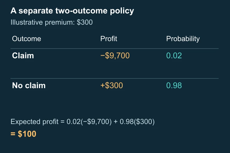
A separate $300-premium, two-outcome insurance distribution: profits −9700 and 300 with probabilities 0.02 and 0.98, giving expected profit 100.

Question 1 of 5

A random variable \(X\) has the distribution: \(P(X=1) = 0.3\), \(P(X=2) = 0.5\), \(P(X=3) = 0.2\). What is \(E(X)\)?

Question 2 of 5

If \(X\) has mean \(\mu_X = 10\) and standard deviation \(\sigma_X = 3\), and \(Y = 2X + 5\), what is \(\sigma_Y\)?

Question 3 of 5

If \(X\) and \(Y\) are independent with \(\sigma_X = 4\) and \(\sigma_Y = 3\), what is the standard deviation of \(X - Y\)?

Question 4 of 5

A random variable \(X\) has \(\mu_X = 50\) and \(\sigma_X = 8\). If you create \(Y = X + 12\), what are \(\mu_Y\) and \(\sigma_Y\)?

Question 5 of 5

Which of the following statements about the variance of a random variable is FALSE?