Introducing Statistics
Random & Non-Random Patterns
Learn to distinguish between random variation and systematic patterns in data: the foundational skill for every statistical inference.
What Is Statistics?
Statistics is the science of collecting, organizing, analyzing, and interpreting data to make informed decisions. At its core, statistics asks one question: is what we see in data real, or just noise?
Random vs Non-Random Patterns
When we observe data, every dataset contains some amount of variability. The key question: is that variability random (due to chance) or does it follow a systematic pattern?
Visualizing Randomness
Below are two scatterplots. One shows random variation around a mean; the other reveals a clear upward trend. Can you tell which is which?
Key Terminology
The Core Principle
This is the foundation of statistical inference. We compare what we observe against what we would expect from a purely random process. If reality deviates far from the expectation, the deviation is likely non-random.
Probability and Randomness
A random process produces outcomes governed by probability. While individual outcomes are unpredictable, the long-run behavior follows a stable distribution described by the Law of Large Numbers.
Types of Non-Random Patterns
Non-random patterns come in several recognizable forms. Learning to identify them is a critical skill in statistics.
Comparing Random and Non-Random
| Random | Non-Random | |
|---|---|---|
| Predictability | Cannot predict individual outcomes | Future values can be anticipated |
| Structure | No detectable pattern | Trend, cycle, cluster, or shift |
| Cause | Natural chance variation | Systematic factor or influence |
| Residuals | Scatter evenly around zero | Show a pattern (curved, grouped) |
| Statistical Action | Variation is expected | Investigate: something is going on |
How to Identify Patterns
Example 1: Fair Coin Flips
A student flips a coin 20 times and records: H T T H H T H T T H T H H T H T T H T H. Is this sequence random?
Example 2: A Suspicious Coin
Another student flips a coin 20 times and gets: H H H H H H H H T H H H H H H T H H H H. That is 18 heads out of 20. Is this random?
Example 3: Reading a Residual Plot
After fitting a linear model to data, we plot the residuals (observed \( - \) predicted). A good model produces residuals that look randomly scattered.
The Runs Test Idea
A run is a consecutive sequence of the same outcome. In the sequence H H T T T H, there are 3 runs: (HH), (TTT), (H). Counting runs helps test for randomness.
Common Mistakes
Summary of Key Concepts
| Concept | What It Means | How to Detect |
|---|---|---|
| Random Variation | Natural, unpredictable fluctuation | Data scatter evenly, no structure |
| Non-Random Pattern | Systematic, predictable structure | Trends, clusters, cycles in plots |
| Law of Large Numbers | Averages stabilize with more data | Proportions converge over time |
| Residual Analysis | Check model fit via residuals | Plot residuals: random = good fit |
| Runs Test | Count consecutive same-type values | Too few or too many runs = non-random |
Worked Example: Detecting a Non-Random Pattern
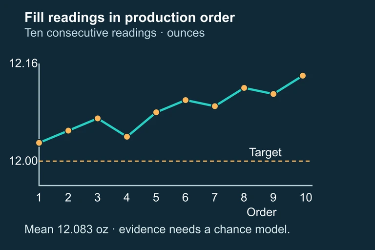
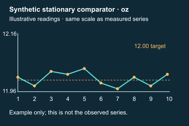
A quality control engineer at a bottling plant measures the fill volume (in ounces) of 10 consecutive bottles from the production line. The target fill is 12.00 oz. The measured values are: 12.03, 12.05, 12.07, 12.04, 12.08, 12.10, 12.09, 12.12, 12.11, 12.14. She wants to determine whether these data suggest a random process centered at 12.00 oz, or whether there is a non-random upward trend indicating that the machine is drifting out of calibration. Analyzing Bottle Fill Data for Non-Random Patterns Step 1 — Compute the Sample Mean We first calculate the sample mean to see where the data are centered. x̄ = (12.03 + 12.05 + 12.07 + 12.04 + 12.08 + 12.10 + 12.09 + 12.12 + 12.11 + 12.14) ÷ 10 = 120.83 ÷ 10. x̄ = 12.083 oz Step 2 — Examine the Deviations from Target All ten observations exceed 12.00 oz, with deviations +0.03,+0.05,+0.07,+0.04,+0.08,+0.10,+0.09,+0.12,+0.11,+0.14. If the deviations are independent and P(fill > 12.00) = 1/2, the probability that all ten are positive is (1/2)¹⁰ = 1/1024 ≈ 0.000977. A mean of 12.00 by itself does not imply equal probabilities above and below the target. Under independent fair-sign assumptions: P(all ten above) = 1/1024. Step 3 — Check for Trend In order, the readings generally rise from 12.03 to 12.14 oz, with local dips. This describes the observed sample; assessing how surprising its trend is requires a specified chance model. The supplemental comparison is synthetic and is not an additional observed sample. Upward trend detected: first observation = 12.03, last observation = 12.14 (increase of 0.11 oz) Step 4 — Interpret the Results All ten readings are above target, the sample mean is 12.083 oz, and the sequence generally rises. These observations warrant investigating the process and checking a justified chance model. Under the independent fair-sign model, ten positive deviations are unlikely, but this sample alone does not identify the cause or establish that immediate recalibration is the appropriate intervention. Observed upward pattern: investigate the process and model assumptions before diagnosing a cause.
Question 1 of 5
A researcher plots residuals from a linear regression and observes that they form a clear curved pattern. What does this indicate?
Question 2 of 5
A coin is flipped 100 times and lands on heads 72 times. The proportion of heads is \( \hat{p} = 0.72 \). Which best describes this result?
Question 3 of 5
Which of the following sequences of coin flips is most consistent with a random process?
Question 4 of 5
The Law of Large Numbers states that as the number of trials increases:
Question 5 of 5
A sequence has \( n_1 = 8 \) values above the median and \( n_2 = 8 \) values below. The expected number of runs is \( E(R) = \frac{2(8)(8)}{16} + 1 = 9 \). If the observed number of runs is 3, what is the most likely conclusion?