Are My Results
Unexpected?
Learn how statisticians determine whether observed outcomes are surprising or simply the result of random chance.
What Does "Unexpected" Mean in Statistics?
In everyday life, we constantly judge whether outcomes are surprising. If you flip a coin 10 times and get 10 heads in a row, you would probably be shocked. But if you got 6 heads, you might shrug it off.
Statistics gives us a formal framework to decide: is an observed result so far from what we expected that it is unlikely to have happened by chance alone?
Expected vs. Observed Outcomes
Variability and the Bell Curve
When we repeat an experiment many times, results cluster around the expected value but vary due to random chance. This spread of possible outcomes forms a distribution.
The Null Hypothesis \( H_0 \)
To decide whether a result is unexpected, we first need a baseline assumption to compare against. In statistics, this is called the null hypothesis (\( H_0 \)).
We also define an alternative hypothesis (\( H_a \)) that captures what we suspect might be true instead: for example, \( H_a: p \neq 0.5 \) (the coin is biased).
The \( p \)-value: Measuring Surprise
The \( p \)-value quantifies how surprising our observed data would be if the null hypothesis were true.
The Significance Level \( \alpha \)
Before collecting data, we choose a threshold called the significance level (\( \alpha \)) to decide what counts as "unexpected enough."
Statistical vs. Practical Significance
A result can be statistically significant (unlikely by chance) without being practically significant (meaningful in the real world). These are different questions.
| Statistical Significance | Practical Significance | |
|---|---|---|
| Question | Is the result unlikely by chance? | Is the result large enough to matter? |
| Measured by | \( p \)-value | Effect size, context |
| Example | A drug lowers blood pressure by 0.5 mmHg (\( p = 0.01 \)) | Is 0.5 mmHg clinically meaningful? Probably not. |
| Depends on | Sample size, variability | Domain knowledge, stakes |
How to Determine if Results Are Unexpected
Example 1: The Coin Flip Test
You flip a coin 100 times and get 62 heads. Is this coin fair?
Visualizing the Coin Flip Result
Example 2: A Not-So-Surprising Result
You flip the same coin 100 times and this time get 53 heads. Is this unexpected?
Example 3: Sample Size Matters
Now suppose you flip the coin 1000 times and get 530 heads (\( \hat{p} = 0.53 \)). Same proportion as before: is it unexpected now?
Why Does This Logic Work?
Common Mistakes to Avoid
Summary: Key Concepts at a Glance
| Concept | Symbol | What It Means |
|---|---|---|
| Null Hypothesis | \( H_0 \) | Baseline: nothing unusual is happening |
| Alternative Hypothesis | \( H_a \) | The claim you want to find evidence for |
| \( p \)-value | \( p \) | Probability of data this extreme under \( H_0 \) |
| Significance Level | \( \alpha \) | Threshold for "unexpected" (usually 0.05) |
| Reject \( H_0 \) | \( p < \alpha \) | Evidence suggests \( H_0 \) is false |
| Fail to Reject \( H_0 \) | \( p \geq \alpha \) | Not enough evidence to reject \( H_0 \) |
Worked Example: Is This Die Fair?
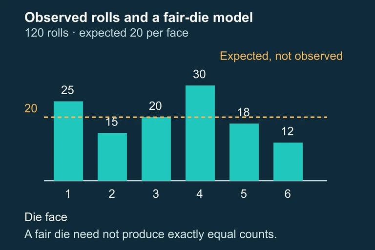
Let us return to the die-rolling scenario from Section 3. You suspect a six-sided die may be loaded, so you roll it 120 times and record the following frequencies: Face 1 → 25, Face 2 → 15, Face 3 → 20, Face 4 → 30, Face 5 → 18, Face 6 → 12. Perform a chi-square goodness-of-fit test at the α = 0.05 significance level. Chi-Square Goodness-of-Fit: Fair Die Step 1 — State Hypotheses H₀: The die is fair; each face has probability p = 1/6. Hₐ: The die is not fair; at least one face has a probability different from 1/6. Step 2 — Check Conditions Assume the 120 rolls are independent (reasonable for a physical die). Each expected count is E = 120 × (1/6) = 20, which satisfies the requirement that all expected counts be at least 5. The conditions for a chi-square goodness-of-fit test are met. All expected counts = 20 ≥ 5 ✓ Step 3 — Compute the Chi-Square Statistic χ² = (25 − 20)²/20 + (15 − 20)²/20 + (20 − 20)²/20 + (30 − 20)²/20 + (18 − 20)²/20 + (12 − 20)²/20 = 25/20 + 25/20 + 0/20 + 100/20 + 4/20 + 64/20 = 1.25 + 1.25 + 0 + 5.00 + 0.20 + 3.20 = 10.90 χ² = 10.90 Step 4 — Determine Degrees of Freedom & P-Value df = k − 1 = 6 − 1 = 5. Using a calculator: χ²cdf(10.90, 1E99, 5) ≈ 0.0534. Alternatively, consulting a chi-square table, the critical value for df = 5 at α = 0.05 is 11.07. p-value ≈ 0.0534, df = 5 Step 5 — State the Conclusion in Context Since the p-value (≈ 0.0534) is greater than α = 0.05, we fail to reject H₀. There is not sufficient evidence at the 5% significance level to conclude that the die is unfair. While the deviations are noticeable—particularly for faces 4 and 6—they are not statistically significant by this standard. Note, however, that the result is borderline; a researcher using α = 0.10 would reject H₀. Fail to reject H₀ at α = 0.05. Insufficient evidence that the die is unfair.
Question 1 of 5
A researcher tests whether a die is fair by rolling it 600 times. She observes 115 sixes. If the die is fair, the expected number of sixes is 100. What is the null hypothesis?
Question 2 of 5
A test yields a \( p \)-value of 0.03. At the \( \alpha = 0.05 \) significance level, what should you conclude?
Question 3 of 5
Which of the following is a correct interpretation of a \( p \)-value of 0.02?
Question 4 of 5
Two studies test the same hypothesis. Study A has \( n = 50 \) and Study B has \( n = 5000 \). Both observe the same sample proportion \( \hat{p} = 0.54 \) under \( H_0: p = 0.50 \). Which study is more likely to reject \( H_0 \)?
Question 5 of 5
A researcher fails to reject \( H_0 \) at the \( \alpha = 0.05 \) level. Which statement is most accurate?