01 / 21

Inference and
Experiments

Learn how to draw causal conclusions from randomized experiments using hypothesis tests for the difference of two means and two proportions.

AP Statistics

Why Experiments Matter

In statistics, the design of a study determines the scope of conclusions we can draw. Only a well-designed randomized experiment allows us to establish a cause-and-effect relationship between variables.

Experiment
Researchers impose a treatment on subjects. Random assignment controls for confounding variables.
Observational Study
Researchers observe existing conditions. No treatment is imposed, so confounders may lurk.

Anatomy of a Randomized Experiment

Subjects Random Assignment Treatment Group 1 Control Group 2 Compare

Key Terms in Experimental Inference

Null Hypothesis \(H_0\)
There is no difference between treatment and control: the treatment has no effect.
Alternative \(H_a\)
There is a difference: the treatment produces a real effect on the response.
\(p\)-value
The probability of observing results at least as extreme as the data, assuming \(H_0\) is true.

A listening study with fixed response cards and moving treatment badges

Participants wear headphones at matching task stations while a researcher distributes cards.Random assignment determines which rearrangements belong in an experimental comparison. Independent groups and measurements linked to the same people require different treatment of the data.

Keep responses fixed while labels change
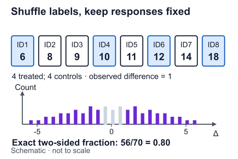
Eight fixed response cards retain their values while four treatment labels are reassigned; an exact randomization distribution marks 56 of 70 assignments.Suppose eight responses are 6, 8, 9, 10, 11, 12, 14 and 18. Under a sharp no-effect null, all 70 assignments of four treatment labels preserve those responses. The observed difference is 1; 56 assignments have an absolute difference at least 1, giving 56/70 = 0.8.

The Two-Sample \(t\)-Test for Means

When comparing two group means from an experiment, the test statistic is:

1
Numerator: the observed difference in sample means \(\bar{x}_1 - \bar{x}_2\) minus the hypothesized difference (usually 0).
2
Denominator: the standard error of the difference, combining variability from both samples.
3
Degrees of freedom: use technology or the conservative \(\min(n_1 - 1,\, n_2 - 1)\).

The Two-Proportion \(z\)-Test

When comparing two group proportions, we pool the proportions under \(H_0\) and use:

Experiments vs. Observational Studies

Experiment Observational Study
Treatment Imposed by researcher Not imposed
Random Assignment Yes No
Confounding Controlled by randomization May be present
Conclusion Causation Association only
Generalization Depends on random selection Depends on random selection

Checking Conditions for Inference

1
Random: Subjects were randomly assigned to treatment groups (this is the hallmark of an experiment).
2
Independent: Individual observations are independent. The 10% condition usually does not apply to experiments (no sampling from a population).
3
Normal (means): Both groups have \(n \geq 30\) or the sample data show no strong skew/outliers.
4
Normal (proportions): The Large Counts condition: \(n_1\hat{p}_c \geq 10\), \(n_1(1-\hat{p}_c) \geq 10\), and the same for group 2.

Step-by-Step Inference Procedure

1
State hypotheses: Write \(H_0\) (no difference) and \(H_a\) (there is a difference). Define parameters clearly.
2
Check conditions: Random assignment? Independence? Normality (CLT or Large Counts)?
3
Calculate: Compute the test statistic (\(t\) or \(z\)) and find the \(p\)-value using technology or tables.
4
Conclude: Compare \(p\)-value to \(\alpha\). If \(p\)-value < \(\alpha\), reject \(H_0\). State the conclusion in context with a causal statement (because it is an experiment).

Example 1: Comparing Means

A researcher randomly assigns 60 students to two groups: 30 use a new study app, 30 use traditional methods. After 4 weeks, test scores are recorded.

App Group
\(\bar{x}_1 = 78.2\), \(s_1 = 8.4\), \(n_1 = 30\)
Traditional
\(\bar{x}_2 = 73.5\), \(s_2 = 9.1\), \(n_2 = 30\)

Example 1: Solution

1
Conditions: Random assignment ✓. Independent groups ✓. Both \(n = 30\), so CLT applies for Normality ✓.
2
Test statistic: \(t = \dfrac{78.2 - 73.5}{\sqrt{\frac{8.4^2}{30} + \frac{9.1^2}{30}}} = \dfrac{4.7}{\sqrt{2.352 + 2.7603}} = \dfrac{4.7}{2.261} \approx 2.079\)
3
\(p\)-value: Using \(df \approx 57\), \(P(t > 2.079) \approx 0.021\)

Example 2: Comparing Proportions

A pharmaceutical company randomly assigns 200 patients to receive either a new drug (100 patients) or a placebo (100 patients). After treatment, 68 of the drug group recovered vs. 52 in the placebo group.

Drug Group
\(\hat{p}_1 = 68/100 = 0.68\), \(n_1 = 100\)
Placebo
\(\hat{p}_2 = 52/100 = 0.52\), \(n_2 = 100\)

Example 2: Solution

1
Pooled proportion: \(\hat{p}_c = \dfrac{68 + 52}{100 + 100} = 0.60\)
2
Conditions: Random assignment ✓. Independent ✓. Large Counts: \(100(0.60)=60 \geq 10\), \(100(0.40)=40 \geq 10\) for both groups ✓.
3
Test statistic: \(z = \dfrac{0.68 - 0.52}{\sqrt{0.60(0.40)\left(\frac{1}{100}+\frac{1}{100}\right)}} = \dfrac{0.16}{\sqrt{0.0048}} = \dfrac{0.16}{0.0693} \approx 2.31\)
4
\(p\)-value: \(P(z > 2.31) \approx 0.0104\)

Writing a Conclusion in Context

A strong AP conclusion has four components:

1
Decision: "Because the \(p\)-value of ___ is less than \(\alpha = 0.05\), we reject \(H_0\)."
2
Evidence statement: "There is convincing evidence that..."
3
Causal language (experiments only): "...the treatment causes / leads to..."
4
Context: Name the specific variables, subjects, and treatments from the problem.

Type I and Type II Errors

Reality
\(H_0\) True
\(H_0\) False
Decision
Reject \(H_0\)
Fail to Reject
Type I Error (False Positive) Correct! Correct! Type II Error (False Negative)
P(Type I) = \(\alpha\)
P(Type II) = \(\beta\)

Common Mistakes

✕ Claiming Causation from Observational Data
Only randomized experiments with random assignment support causal conclusions. Observational studies show association only.
✕ Forgetting to Pool Proportions
For a two-proportion \(z\)-test, you must use the pooled \(\hat{p}_c\) in the standard error, not individual \(\hat{p}\) values.
✕ Accepting \(H_0\)
We never "accept" the null. We either reject \(H_0\) or fail to reject \(H_0\). Absence of evidence is not evidence of absence.

Question 1 of 5

A researcher randomly assigns 50 volunteers to a new exercise program and 50 to a control group. After 8 weeks, the exercise group lost significantly more weight (\(p\)-value = 0.003). Which conclusion is most appropriate?

Question 2 of 5

In a two-proportion \(z\)-test for an experiment, why do we use a pooled proportion \(\hat{p}_c\) rather than the individual sample proportions?

Question 3 of 5

A two-sample \(t\)-test yields a \(p\)-value of 0.08 at \(\alpha = 0.05\). Which statement is correct?

Question 4 of 5

A study finds that coffee drinkers have lower rates of depression than non-coffee drinkers (\(p = 0.01\)). The data were collected from a large random sample survey. What is the strongest valid conclusion?

Question 5 of 5

In a randomized experiment, a researcher rejects \(H_0\) at \(\alpha = 0.05\). If \(H_0\) is actually true, what type of error has been made?