Estimating Probabilities
Using Simulation
Learn to use random processes and repeated trials to estimate probabilities when theoretical calculations are complex or impossible.
What Is a Simulation?
A simulation is an imitation of a real-world random process using a model. Instead of performing the actual experiment (which may be costly, dangerous, or impossible), we use tools like random number generators, coins, dice, or cards to mimic the process many times.
Why Simulate Instead of Calculate?
The Law of Large Numbers
The Law of Large Numbers states that as the number of trials \( n \) increases, the empirical (observed) proportion of an event converges to the event's true probability:
Key Vocabulary
Theoretical vs. Empirical Probability
| Theoretical | Empirical (Simulated) | |
|---|---|---|
| Definition | Based on mathematical reasoning about equally likely outcomes | Based on observed results from repeated trials |
| Formula | \(\frac{\text{favorable outcomes}}{\text{total outcomes}}\) | \(\frac{\text{occurrences of event}}{n}\) |
| Requirements | All outcomes must be equally likely and countable | Only needs a repeatable random process |
| Accuracy | Exact | Approximate (improves with more trials) |
| Example | \(P(\text{heads}) = 0.5\) for a fair coin | Flip 1000 times, get 507 heads: \(\hat{p} = 0.507\) |
How to Design a Simulation
Example 1: Free Throw Streaks
A basketball player makes 80% of her free throws. What is the probability she makes all 5 free throws in a game?
Checking with Theory
Since each free throw is independent with \( P(\text{make}) = 0.80 \), the theoretical probability of making all 5 is:
Our simulation estimate of \(\hat{p} = 0.34\) is close to the theoretical value of 0.328. With more trials, the estimates would converge even closer. This validates both the simulation design and the theoretical answer.
Example 2: The Birthday Problem
In a class of 25 students, what is the probability that at least two share the same birthday? This is surprisingly hard to calculate by hand, but easy to simulate.
Example 3: Cereal Box Collector
A cereal brand puts one of 6 different toys in each box (equally likely). How many boxes must you buy on average to collect all 6 toys?
Ten cereal boxes, five collectible prizes, and one changing stopping rule
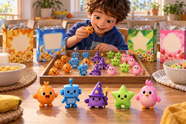 Collecting all prize types and waiting for the first designated prize use different stopping rules. Define the response variable before generating trials.
Define completion by ten boxes
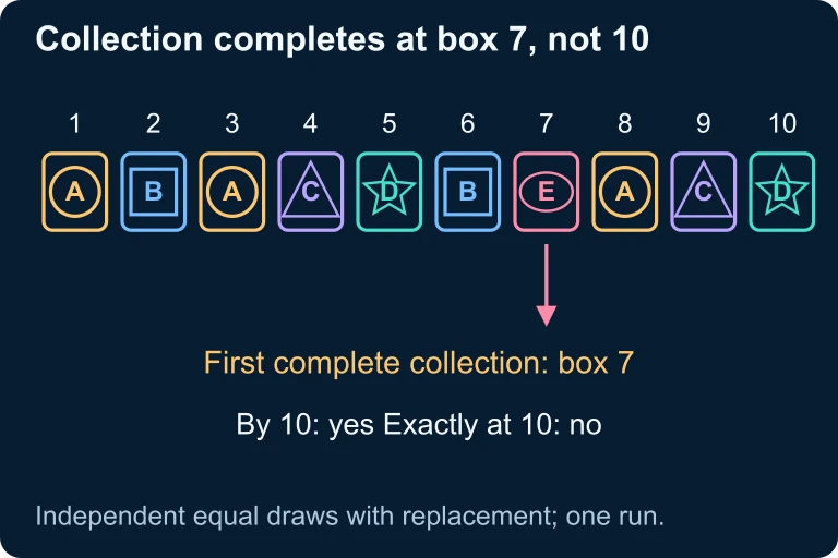 Suppose each box independently contains one of five equally likely prize types. In the sequence A, B, A, C, D, B, E, A, C, D, all five types first appear at box 7. This trial succeeds for completion by ten boxes; repeated trials estimate the event’s probability.
Repeated prizes still count as trials
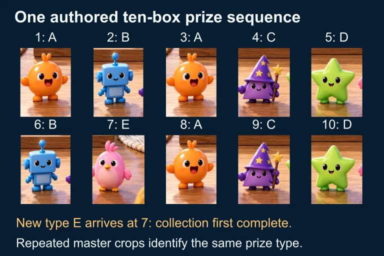 The ten-box sequence is A, B, A, C, D, B, E, A, C, D. New types increase the collection count; repeated types leave it unchanged. Start a fresh collection for the next trial.
Choosing a Random Device
| Probability | Random Device | Mapping |
|---|---|---|
| \(P = 0.50\) | Coin flip | Heads = success, Tails = fail |
| \(P = 1/6\) | Single die | Roll 1 = success, 2-6 = fail |
| \(P = 0.80\) | Digits 0-9 | 1-8 = success, 9, 0 = fail |
| \(P = 0.35\) | Digits 00-99 | 01-35 = success, 00 & 36-99 = fail |
| \(P = 0.417\) | Digits 000-999 | 001-417 = success, 000 & 418-999 = fail |
How Many Trials Are Enough?
More trials yield more accurate estimates. But how many is "enough"? The margin of error for an estimated proportion decreases as:
Using a Random Number Table
On the AP exam, you may be given a table of random digits. Here's how to use it for a simulation where \( P = 0.70 \):
Common Mistakes to Avoid
Summary of Simulation Steps
| Step | Action | Example (Free Throws) |
|---|---|---|
| 1. Component | Identify one random element | One free throw attempt |
| 2. Assign | Map outcomes to random device | Digits 1-8 = make, 9,0 = miss |
| 3. Trial | Define one full experiment | 5 consecutive digits |
| 4. Response | What to record | Did all 5 digits fall in 1-8? |
| 5. Repeat | Run many trials | 50+ trials, compute \(\hat{p}\) |
Question 1 of 5
A simulation of 200 trials is used to estimate a probability. In 68 of those trials, the event occurred. What is the estimated probability of the event?
Question 2 of 5
A player makes 60% of her penalty kicks. To simulate this, you use single random digits 0-9. Which assignment is correct?
Question 3 of 5
Why does a simulation with 1000 trials generally give a better estimate than one with 50 trials?
Question 4 of 5
To estimate the probability that a couple with 3 children has all boys (assuming \(P(\text{boy}) = 0.5\)), what constitutes one trial in the simulation?
Question 5 of 5
A student runs a simulation and gets \(\hat{p} = 0.42\) based on 500 trials. Using the approximation \(\text{ME} \approx \frac{1}{\sqrt{n}}\), the margin of error is approximately: