Difference of Two Means
Setting Up the Test
Learn how to set up a hypothesis test comparing two population means: defining hypotheses, checking conditions, and computing the test statistic.
What Is a Two-Sample \(t\)-Test?
When we have data from two independent groups, we often want to know whether their population means are different. A two-sample \(t\)-test compares \(\mu_1\) and \(\mu_2\) by examining the difference \(\bar{x}_1 - \bar{x}_2\).
Two Populations, Two Samples
Why Does This Matter?
In every case, we need a structured test: state hypotheses, verify conditions, compute a statistic, and make a decision. Let's learn the setup.
Step 1: State the Hypotheses
The alternative hypothesis reflects the research question. Choose the direction before collecting data.
Step 2: Check the Conditions
Step 3: The Test Statistic
Degrees of Freedom
The two-sample \(t\)-test does not use a simple formula for degrees of freedom. On the AP exam, you have two options:
Paired vs. Two-Sample
| Two-Sample \(t\) | Paired \(t\) | |
|---|---|---|
| Samples | Independent groups | Matched pairs or before/after |
| Data | Two separate lists of values | One list of differences |
| Parameter | \(\mu_1 - \mu_2\) | \(\mu_d\) (mean difference) |
| SE formula | \(\sqrt{\frac{s_1^2}{n_1} + \frac{s_2^2}{n_2}}\) | \(\frac{s_d}{\sqrt{n}}\) |
| df | Welch's or \(\min(n_1\!-\!1, n_2\!-\!1)\) | \(n - 1\) |
A listening study with fixed response cards and moving treatment badges
 Measurements taken from the same person remain linked. Compare within-person differences instead of treating the two columns as independent samples.
Keep the pairs linked
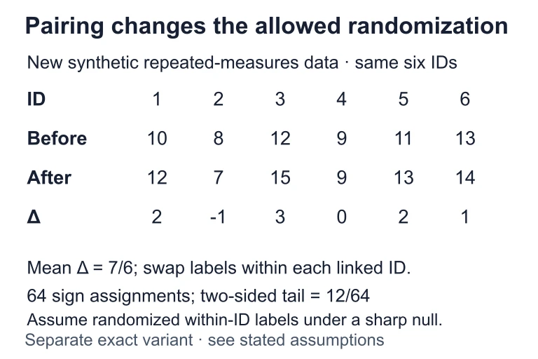 Suppose the same six IDs have differences 2, −1, 3, 0, 2 and 1, averaging 7/6. Under a sharp zero-effect null with randomized or exchangeable within-ID labels, 2⁶ = 64 sign assignments are allowed; 12 have absolute mean at least 7/6. Repeated measurement alone does not establish that exchangeability.
How to Set Up the Test
Example 1: Battery Life
A company tests two battery brands. Brand A: \(n_1 = 35\), \(\bar{x}_1 = 48.2\) hours, \(s_1 = 4.1\). Brand B: \(n_2 = 40\), \(\bar{x}_2 = 45.8\) hours, \(s_2 = 3.7\). Is there a difference at \(\alpha = 0.05\)?
Example 1: Conclusion
Example 2: Exam Scores
A teacher believes her morning class (Class 1) scores higher than her afternoon class (Class 2). Data: \(n_1 = 22\), \(\bar{x}_1 = 78.5\), \(s_1 = 9.3\); \(n_2 = 25\), \(\bar{x}_2 = 75.1\), \(s_2 = 10.8\). Test at \(\alpha = 0.05\).
Example 3: Writing the Full Setup
Researchers compare the mean reaction time (ms) of caffeine users vs. non-users. They collect: \(n_1 = 50\), \(\bar{x}_1 = 245\), \(s_1 = 32\); \(n_2 = 50\), \(\bar{x}_2 = 262\), \(s_2 = 38\). They believe caffeine users react faster (lower mean).
Common Mistakes
Setup Summary
| Component | What to Write |
|---|---|
| Parameter | Define \(\mu_1\) and \(\mu_2\) in context |
| Null Hypothesis | \(H_0\!: \mu_1 - \mu_2 = 0\) |
| Alt. Hypothesis | \(H_a\!: \mu_1 - \mu_2 \neq / \lt / \gt 0\) |
| Conditions | Random, Independent (10%), Normal/Large |
| Test Statistic | \(t = \frac{(\bar{x}_1 - \bar{x}_2)}{\sqrt{\frac{s_1^2}{n_1} + \frac{s_2^2}{n_2}}}\) |
| Degrees of Freedom | Calculator (Welch) or \(\min(n_1\!-\!1,\, n_2\!-\!1)\) |
Question 1 of 5
A researcher wants to test whether the mean weight of tomatoes from Farm A is different from the mean weight from Farm B. Which is the correct alternative hypothesis?
Question 2 of 5
Which of the following is not a condition for a two-sample \(t\)-test?
Question 3 of 5
Given: \(\bar{x}_1 = 52\), \(s_1 = 6\), \(n_1 = 36\), \(\bar{x}_2 = 48\), \(s_2 = 8\), \(n_2 = 49\). What is the standard error of \(\bar{x}_1 - \bar{x}_2\)?
Question 4 of 5
Students measure their own heart rates before and after exercise. Each student's "before" is compared to their own "after." Which test is appropriate?
Question 5 of 5
A test yields \(t = -1.82\) with \(df = 38\) for a left-tailed test. Using a \(t\)-table, the \(p\)-value is between 0.025 and 0.05. At \(\alpha = 0.05\), what is the conclusion?