01 / 21

Comparing
Distributions

Learn how to compare distributions of a quantitative variable using shape, center, spread, and unusual features to draw meaningful statistical conclusions.

AP Statistics

What Does It Mean to Compare Distributions?

When we compare distributions, we examine two or more groups measured on the same quantitative variable. The goal is to identify meaningful similarities and differences that reveal patterns or support claims.

Same Variable
Both groups must be measured on the same quantitative scale (e.g., test scores, heights).
Different Groups
Groups are defined by a categorical variable (e.g., male vs. female, treatment vs. control).

The Four Features to Compare

AP Statistics uses the acronym SOCS (or CUSS) to remember what to address when comparing distributions:

Shape
Symmetric, skewed left, skewed right, uniform, bimodal?
Center
Mean or median: which group's "typical value" is higher?
Spread
Range, IQR, or standard deviation: which group is more variable?
Outliers
Any unusual values? Are they present in one group but not the other?

Visualizing Comparisons

Several graphs are useful for comparing distributions side by side. The most common in AP Statistics are:

Side-by-Side Boxplots
Great for comparing center, spread, and outliers at a glance on a common axis.
Back-to-Back Stemplots
Shows individual values and shape for small data sets with two groups.
Parallel Dotplots / Histograms
Stacked or side-by-side on the same scale for direct visual comparison of shape.

The Core Rule for AP Free Response

1
Always compare: use words like "greater," "less," "similar," "more variable."
2
Always use context: name the variable and both groups in your answer.
3
Use numerical values when available (medians, IQRs, etc.) to support comparisons.

Reading Side-by-Side Boxplots

40 60 80 100 120 Test Score A 45 55 75 95 105 B 60 70 90 105 115

Describing Shape in Context

Group A: Skewed Right Group B: Approximately Symmetric

Comparing Center and Spread

Measures of Center
Use the median when distributions are skewed or have outliers. Use the mean when distributions are roughly symmetric.
Measures of Spread
Pair IQR with the median, and standard deviation (\( s \)) with the mean. Report the measure that matches your center.

Describing vs. Comparing

Describing (One Group) Comparing (Two Groups)
Focus One distribution in isolation Similarities and differences between groups
Language "The distribution is..." / "The center is..." "Group A is higher than..." / "...more spread than..."
Features Shape, center, spread, outliers Same features, but stated comparatively
Common Error N/A Describing each group separately without comparing

Step-by-Step Approach

1
Identify the groups and variable. What categorical variable defines the groups? What quantitative variable is being measured?
2
Compare shape. Are both symmetric? Is one skewed while the other is not? Mention modality if relevant.
3
Compare center. Which group has a higher median (or mean)? Use numerical values from the graph.
4
Compare spread. Which group has a larger IQR, range, or standard deviation? Cite numbers.
5
Note outliers. Does either group have outliers? If so, describe them in context.

Worked Example: Battery Life

Battery Life (hours) 2 4 6 8 10 X 5.5 Y 7.0

Worked Example: Commute Times

Commute Time (minutes) 5 15 25 35 45 A outlier B

Comparing with Summary Statistics

Sometimes you are given a table of statistics instead of a graph. You still compare the same four features.

School A School B
Mean 72.3 78.1
Median 74 79
Std Dev (\( s \)) 12.5 8.2
IQR 18 11
Shape Slightly left-skewed Approximately symmetric

Resistant vs. Non-Resistant Measures

Choosing the right summary statistic matters when distributions have different shapes or outliers:

Resistant (Robust)
Median and IQR: not heavily affected by outliers or skewness. Preferred when distributions are skewed.
Non-Resistant
Mean and standard deviation: pulled by extreme values. Best for approximately symmetric distributions without outliers.

Common Mistakes to Avoid

✕ Describing Instead of Comparing
Writing "Group A is skewed right. Group B is symmetric." without explicit comparison loses points on the AP exam.
✕ Forgetting Context
Saying "the median is higher" without naming the variable (e.g., "battery life") and groups (e.g., "Brand X") is incomplete.
✕ Mismatched Statistics
Comparing the mean of one group to the median of another. Always use the same measure for both groups.

Summary Checklist

Feature What to Say Key Statistics
Shape "Both are symmetric" / "A is skewed, B is not" Visual assessment
Center "Group A's median is higher than Group B's" Mean or Median
Spread "Group A is more variable than Group B" IQR, \( s \), or Range
Outliers "Group A has an outlier at 98; Group B has none" \( Q_1 - 1.5 \times \text{IQR} \) rule
Context Name the variable and both groups Always required

Worked Example: Comparing Two Groups

A researcher collected data on the number of hours of sleep per night for two groups: 12 college students during finals week and 12 college students during a regular (non-exam) week. The data are summarized below. Statistic | Finals Week | Regular Week Minimum | 3.5 | 6.0 Q₁ | 4.5 | 6.8 Median | 5.5 | 7.5 Q₃ | 6.2 | 8.0 Maximum | 7.0 | 9.0 Mean | 5.3 | 7.4 Std. Dev. | 1.1 | 0.9 Writing a Complete Comparison (SOCS) Step 1 — Compare Shape For the finals week group, the mean (5.3) is slightly less than the median (5.5), suggesting a slight left skew—some students may have gotten very little sleep. For the regular week group, the mean (7.4) and median (7.5) are nearly equal, suggesting a roughly symmetric distribution. Both distributions are approximately symmetric to slightly skewed. Both distributions are roughly symmetric; the finals week group may be slightly left-skewed. Step 2 — Note Outliers / Unusual Features Using the 1.5 × IQR rule for the finals group: IQR = 6.2 − 4.5 = 1.7, so fences are at 4.5 − 1.5(1.7) = 1.95 and 6.2 + 1.5(1.7) = 8.75. The minimum (3.5) and maximum (7.0) both fall within these fences, so there are no outliers. For the regular week group: IQR = 8.0 − 6.8 = 1.2, fences at 6.8 − 1.8 = 5.0 and 8.0 + 1.8 = 9.8. Again, no outliers. Neither distribution appears to have outliers by the 1.5 × IQR criterion. Step 3 — Compare Center The median sleep during finals week (5.5 hours) is substantially lower than the median sleep during a regular week (7.5 hours)—a difference of 2.0 hours. This indicates that college students typically get about 2 fewer hours of sleep per night during finals compared to a normal week. Center: Regular week median (7.5 hrs) is 2.0 hours higher than finals week median (5.5 hrs). Step 4 — Compare Spread The IQR for the finals week group (1.7 hours) is greater than the IQR for the regular week group (1.2 hours), and the standard deviations tell the same story (1.1 vs. 0.9). The range of sleep hours during finals (3.5 hours) also exceeds that of a regular week (3.0 hours). This suggests that there is more variability in sleep during finals week—some students cut sleep dramatically while others maintain closer-to-normal patterns. Spread: Finals week (IQR = 1.7, s = 1.1) is more variable than regular week (IQR = 1.2, s = 0.9). Step 5 — Context & Conclusion In the context of this study, college students during finals week get substantially less sleep and show more variability in sleep hours than students during a regular week. The distributions have similar shapes (both roughly symmetric) and neither contains outliers, but they differ meaningfully in center and spread. Complete comparison: Both distributions are roughly symmetric with no outliers, but finals-week sleep is centered about 2 hours lower and is more variable than regular-week sleep.
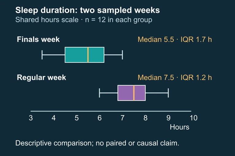
Independent-group boxplots on a common scale, each with n=12. Medians are 5.5 and 7.5; interquartile ranges are 1.7 and 1.2.
The sampled finals-week group has a lower median and a larger IQR than the regular-week group; summaries do not establish causation or full shape.
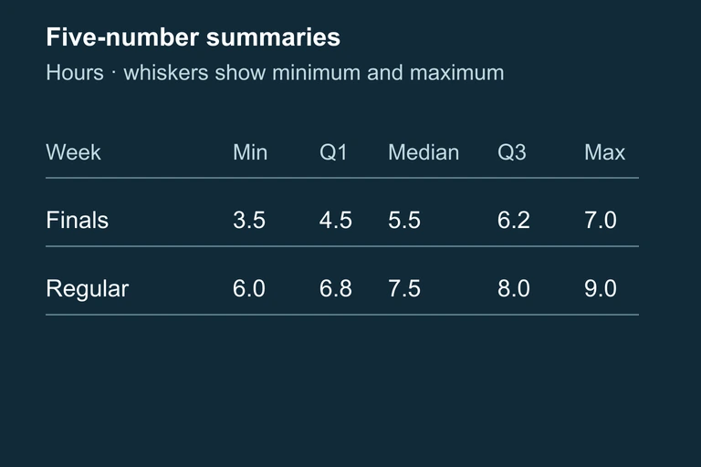
Table of both groups’ five-number summaries. Boxplot whiskers represent minimum and maximum values.

Question 1 of 5

When comparing two distributions, which set of features should you always address?

Question 2 of 5

A student writes: "Group A has a median of 50. Group B has a median of 65." Why would this response not receive full credit on an AP exam?

Question 3 of 5

Distribution X is strongly skewed right with several high outliers. Distribution Y is approximately symmetric. Which pair of statistics is most appropriate to compare their centers and spreads?

Question 4 of 5

Two side-by-side boxplots show that Group A's box is entirely to the left of Group B's box (with no overlap). What can you conclude?

Question 5 of 5

Group A has \( \text{IQR} = 22 \) and Group B has \( \text{IQR} = 10 \). Group A's range is 40 and Group B's range is 55. Which statement best compares their spreads?