Combining
Random Variables
Learn the rules for finding the mean and variance when you add, subtract, or scale random variables: the foundation of inference in statistics.
What Is a Random Variable?
A random variable assigns a numerical value to each outcome of a random process. It is described by its probability distribution, which tells us what values it can take and how likely each value is.
Why Combine Random Variables?
In real life, outcomes often depend on more than one random quantity. Combining them lets us predict the behavior of totals, differences, and scaled measurements.
Linear Transformations: \(a + bX\)
When you shift by a constant \(a\) and scale by a constant \(b\), the mean and variance change predictably:
Core Rules: Sums and Differences
\(\mu_{X+Y} = \mu_X + \mu_Y\) and \(\mu_{X-Y} = \mu_X - \mu_Y\)
\(\sigma_{X+Y}^2 = \sigma_X^2 + \sigma_Y^2\) and \(\sigma_{X-Y}^2 = \sigma_X^2 + \sigma_Y^2\)
\(\sigma_{X+Y} = \sqrt{\sigma_X^2 + \sigma_Y^2}\)
Variance Always Adds
The Independence Requirement
The variance addition rule only works when \(X\) and \(Y\) are independent. If they are not independent, a covariance term appears:
\(X_1 + X_2\) vs \(2X\)
These look similar but are fundamentally different. One involves two independent observations; the other scales a single observation.
| \(X_1 + X_2\) | \(2X\) | |
|---|---|---|
| Meaning | Sum of two independent draws | Double one single draw |
| Mean | \(\mu + \mu = 2\mu\) | \(2\mu\) |
| Variance | \(\sigma^2 + \sigma^2 = 2\sigma^2\) | \(4\sigma^2\) |
| Std Dev | \(\sigma\sqrt{2}\) | \(2\sigma\) |
A filling line that deposits one statistic for a whole tray
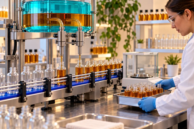
A production line can combine two independent measurements or scale one measurement. Those operations can share a mean while producing different variances.Double one draw or add independent draws
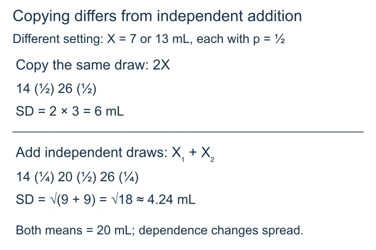
Suppose X is equally likely to be 7 or 13. Then 2X is 14 or 26 and has standard deviation 6. For independent X₁ and X₂, their sum is 14, 20 or 26 with probabilities 1/4, 1/2 and 1/4 and standard deviation √18. Both means are 20.How to Apply the Rules
Example 1: Adding Two Tests
A student's math score \(M\) has \(\mu_M = 520\), \(\sigma_M = 115\). Their verbal score \(V\) has \(\mu_V = 480\), \(\sigma_V = 110\). Scores are independent. Find the mean and standard deviation of \(T = M + V\).
Example 2: Difference of Variables
A factory produces bolts with diameter \(B\): \(\mu_B = 10\,\text{mm}\), \(\sigma_B = 0.3\,\text{mm}\), and nuts with hole diameter \(N\): \(\mu_N = 10.2\,\text{mm}\), \(\sigma_N = 0.2\,\text{mm}\). Let \(G = N - B\) (the gap). Find \(\mu_G\) and \(\sigma_G\).
Example 3: Scaling Then Combining
Let \(X\) have \(\mu_X = 50\), \(\sigma_X = 8\), and \(Y\) have \(\mu_Y = 30\), \(\sigma_Y = 6\). \(X\) and \(Y\) are independent. Find the mean and standard deviation of \(W = 3X - 2Y + 10\).
Common Mistakes
Summary of Rules
| Operation | Mean | Variance (indep.) |
|---|---|---|
| \(a + bX\) | \(a + b\mu_X\) | \(b^2 \sigma_X^2\) |
| \(X + Y\) | \(\mu_X + \mu_Y\) | \(\sigma_X^2 + \sigma_Y^2\) |
| \(X - Y\) | \(\mu_X - \mu_Y\) | \(\sigma_X^2 + \sigma_Y^2\) |
| \(aX + bY\) | \(a\mu_X + b\mu_Y\) | \(a^2\sigma_X^2 + b^2\sigma_Y^2\) |
| \(X_1 + X_2\) (iid) | \(2\mu_X\) | \(2\sigma_X^2\) |
| \(2X\) | \(2\mu_X\) | \(4\sigma_X^2\) |
Key Takeaways Before Practice
Worked practice: Practice Problems, Problem 4 — Applied
Work through this original lesson problem, then reveal the solution and illustrations.
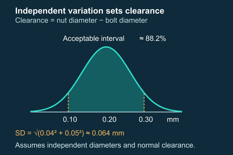
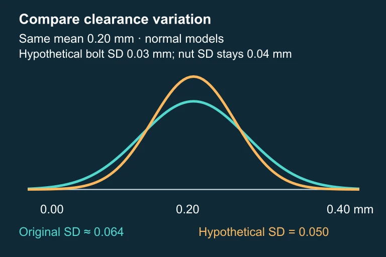
A manufacturing process produces bolts with mean diameter μ_B = 10.00 mm and standard deviation σ_B = 0.05 mm, and nuts with mean inner diameter μ_N = 10.20 mm and standard deviation σ_N = 0.04 mm. Bolt and nut diameters are independent. An engineer defines the clearance as C = N − B (nut inner diameter minus bolt diameter). A bolt-nut pair is considered acceptable if the clearance is between 0.10 mm and 0.30 mm. (a) Find the mean and standard deviation of C. (b) Assuming C is approximately normal, find the probability that a randomly selected bolt-nut pair is acceptable. (c) A redesign reduces σ_B to 0.03 mm. Without recalculating the exact probability, explain how this change affects the distribution of C and the proportion of acceptable pairs.
Show answer and explanation
(a) [2 points] μ_C = μ_N − μ_B = 10.20 − 10.00 = 0.20 mm. Since B and N are independent, σ²_C = σ²_N + σ²_B = (0.04)² + (0.05)² = 0.0016 + 0.0025 = 0.0041. Thus σ_C = √0.0041 ≈ 0.0640 mm. (b) [2 points] Use σ_C = √0.0041 ≈ 0.064031242 mm without premature rounding. Then z_low = −0.1/√0.0041 ≈ −1.561737619 and z_high ≈ 1.561737619. Thus P(0.10 < C < 0.30) = 2Φ(1.561737619) − 1 ≈ 0.881650. About 88.2% of pairs are acceptable under the approximate normal model. (c) [2 points] Reducing σ_B decreases the total variance of C. The new σ²_C = (0.04)² + (0.03)² = 0.0025, giving σ_C = 0.05 mm. Since the mean clearance remains 0.20 mm (the center of the acceptable range), a narrower distribution concentrates more area within the acceptable interval, increasing the proportion of acceptable pairs.
Question 1 of 5
If \(X\) and \(Y\) are independent with \(\sigma_X = 3\) and \(\sigma_Y = 4\), what is \(\sigma_{X+Y}\)?
Question 2 of 5
Let \(X\) have \(\mu_X = 20\) and \(\sigma_X^2 = 9\). What are the mean and variance of \(Y = 5 + 3X\)?
Question 3 of 5
Independent random variables \(A\) and \(B\) have means \(\mu_A = 100\) and \(\mu_B = 60\), with variances \(\sigma_A^2 = 25\) and \(\sigma_B^2 = 16\). What is \(\operatorname{Var}(A - B)\)?
Question 4 of 5
A random variable \(X\) has \(\mu_X = 10\) and \(\sigma_X^2 = 5\). Two independent observations \(X_1\) and \(X_2\) are drawn. What is \(\operatorname{Var}(X_1 + X_2)\)?
Question 5 of 5
Which statement is always true for independent random variables \(X\) and \(Y\)?