01 / 21
\(\chi^2\)

Chi-Square
Goodness of Fit Test

Learn how to determine whether observed data matches an expected distribution using the \(\chi^2\) statistic and p-values.

AP Statistics

What Is a Goodness of Fit Test?

A chi-square goodness of fit test asks a simple question: does the distribution of observed counts match what we expected? It compares a single categorical variable's observed frequencies against a hypothesized (expected) distribution.

Observed
The actual counts you collect from data
Expected
The counts predicted by the null hypothesis
\(\chi^2\) Statistic
Measures total deviation between observed and expected

Setting Up the Hypotheses

\(H_0\): Null Hypothesis
The observed distribution matches the expected distribution. There is no significant difference.
\(H_a\): Alternative Hypothesis
The observed distribution does not match the expected distribution. At least one category differs.

Observed vs. Expected: A Visual

0 10 20 30 40 A B C D Observed Expected

The \(\chi^2\) Test Statistic

\(O_i\)
Observed count for category \(i\)
\(E_i\)
Expected count for category \(i\) under \(H_0\)
\(\sum\)
Sum across all \(k\) categories

Each category contributes \(\frac{(O - E)^2}{E}\) to the total. Categories with large deviations from expected contribute more.

Degrees of Freedom

Where \(k\) is the number of categories. For example, if a die has 6 faces, \(df = 6 - 1 = 5\).

Conditions for the \(\chi^2\) Test

1
Random: The data must come from a random sample or randomized experiment.
2
Independent: Individual observations are independent. If sampling without replacement, \(n < 10\%\) of the population (the 10% condition).
3
Large Counts: All expected counts must satisfy \(E_i \geq 5\) for every category. This ensures the \(\chi^2\) approximation is valid.

GOF vs. Other \(\chi^2\) Tests

Goodness of Fit Independence / Homogeneity
Variables One categorical variable Two categorical variables
Compares Observed vs. claimed distribution Observed vs. independence model
Degrees of Freedom \(k - 1\) \((r - 1)(c - 1)\)
Data Layout One-way table Two-way table
Example Is this die fair? Is gender related to preference?

The \(\chi^2\) Distribution

0 3 6 9 12 15
\(\chi^2\)
df = 2 df = 4 df = 8

How to Carry Out the Test

1
State hypotheses: Write \(H_0\) (distribution matches claim) and \(H_a\) (distribution differs).
2
Check conditions: Random, Independent (10% rule), Large Counts (\(E_i \geq 5\)).
3
Compute expected counts: \(E_i = n \times p_i\) where \(p_i\) is the hypothesized proportion for category \(i\).
4
Calculate the test statistic: \(\chi^2 = \sum \frac{(O_i - E_i)^2}{E_i}\) with \(df = k - 1\).
5
Find the p-value: Use the \(\chi^2\) distribution with \(df = k - 1\) (table or calculator).
6
Make a conclusion: If \(p\text{-value} \le \alpha\), reject \(H_0\). State in context.

Example 1: Fair Die?

A student rolls a die 60 times and records the results. She wants to test whether the die is fair at \(\alpha = 0.05\).

Face 1 2 3 4 5 6
Observed 8 12 14 7 9 10
Expected 10 10 10 10 10 10

Example 1: Computation

\(\chi^2 = 3.4\)
Test statistic
\(df = 5\)
\(6 - 1 = 5\)
\(p \approx 0.639\)
Using \(\chi^2\) table or calculator

Example 2: Candy Colors

A candy company claims its bags contain colors in these proportions: Red 30%, Blue 25%, Green 20%, Yellow 15%, Orange 10%. A student samples 200 candies.

Color Red Blue Green Yellow Orange
Observed (\(O\)) 75 42 30 38 15
Expected (\(E\)) 60 50 40 30 20

Example 2: Solution

\(\chi^2 \approx 10.913\)
Test statistic
\(df = 4\)
\(5 - 1 = 4\)
\(p \approx 0.028\)
Between 0.02 and 0.05

Common Mistakes

✕ Using Proportions Instead of Counts
The formula requires raw counts, not percentages. Always compute \(E_i = n \times p_i\) to get counts.
✕ Checking \(\text{Observed} \geq 5\)
The Large Counts condition requires all expected counts \(\geq 5\), not observed counts.
✕ Wrong Degrees of Freedom
Using \(k\) or \(n - 1\) instead of \(k - 1\). Remember: \(df\) is the number of categories minus 1.
✕ Two-Sided Conclusion
Saying "reject because the distribution is higher." The \(\chi^2\) test only tells you the distribution differs, not the direction.

Summary Checklist

✓
One categorical variable, comparing observed to a claimed distribution
✓
\(H_0\): distribution matches claim. \(H_a\): distribution differs
✓
Conditions: Random, Independent (10% rule), Large Counts (\(E_i \geq 5\))
✓
Test statistic: \(\chi^2 = \sum \frac{(O_i - E_i)^2}{E_i}\) with \(df = k - 1\)
✓
Compare p-value to \(\alpha\). Conclude in context

Worked Example: M&M Color Distribution

A statistics student suspects that the color distribution of M&M's in a large bag does not match the company's published percentages. The company claims the following distribution: 24% blue, 20% orange, 16% green, 14% yellow, 13% red, and 13% brown. The student takes a random sample of 200 M&M's and records the following observed counts: Blue = 53, Orange = 38, Green = 35, Yellow = 27, Red = 22, Brown = 25. Carry out a chi-square goodness-of-fit test at the α = 0.05 significance level. (Assume the hypotheses have been stated and conditions verified.) Chi-Square Goodness-of-Fit Test: M&M Color Distribution Step 1 — Compute Expected Counts Multiply the total sample size n = 200 by each hypothesized proportion: E(Blue) = 200 × 0.24 = 48, E(Orange) = 200 × 0.20 = 40, E(Green) = 200 × 0.16 = 32, E(Yellow) = 200 × 0.14 = 28, E(Red) = 200 × 0.13 = 26, E(Brown) = 200 × 0.13 = 26. Verify: 48 + 40 + 32 + 28 + 26 + 26 = 200 ✓. All expected counts are ≥ 5, confirming the conditions are met. Expected counts: 48, 40, 32, 28, 26, 26 Step 2 — Compute Each Component of χ² For each category, compute (O − E)²/E. Blue: (53 − 48)²/48 = 25/48 ≈ 0.5208. Orange: (38 − 40)²/40 = 4/40 = 0.1000. Green: (35 − 32)²/32 = 9/32 ≈ 0.2813. Yellow: (27 − 28)²/28 = 1/28 ≈ 0.0357. Red: (22 − 26)²/26 = 16/26 ≈ 0.6154. Brown: (25 − 26)²/26 = 1/26 ≈ 0.0385. Components: 0.521, 0.100, 0.281, 0.036, 0.615, 0.038 Step 3 — Sum to Get the Test Statistic χ² = 0.5208 + 0.1000 + 0.2813 + 0.0357 + 0.6154 + 0.0385 = 1.5917. Rounding appropriately, χ² ≈ 1.592. χ² = 1.592 Step 4 — Determine Degrees of Freedom and P-Value There are k = 6 categories, so df = 6 − 1 = 5. Using a TI-84 calculator: χ²cdf(1.592, 1E99, 5) ≈ 0.902. Alternatively, looking at a chi-square table, the critical value for α = 0.05 with df = 5 is 11.07; since 1.592 is far below 11.07, the p-value is clearly much larger than 0.05. p-value ≈ 0.902, df = 5 Step 5 — State the Conclusion in Context Because the p-value (0.902) is greater than α = 0.05, we fail to reject H₀. There is not convincing evidence that the distribution of M&M colors in this bag differs from the company's published color distribution. The observed deviations from the claimed percentages are small enough to be plausibly attributed to random sampling variability. Fail to reject H₀. No convincing evidence of a difference. Five-category, 150-candy illustration. This does not replace the separate six-category, 200-candy worked example.
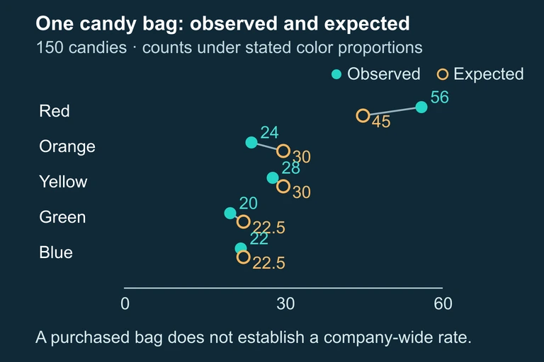
Five observed versus expected candy counts for a 150-candy example. Expected counts include 45,30,30,22.5,22.5. Sampling from one bag does not establish company-wide inference.
Observed color counts from one purchased bag can be compared with the stated model, but this design does not establish company-wide inference.

Question 1 of 5

A researcher claims that four types of cereal are equally popular. She surveys 120 people. What are the expected counts for each cereal type under \(H_0\)?

Question 2 of 5

A chi-square goodness of fit test has 6 categories. What are the degrees of freedom?

Question 3 of 5

In a \(\chi^2\) GOF test, the Large Counts condition requires:

Question 4 of 5

A \(\chi^2\) GOF test yields \(\chi^2 = 15.3\) with \(df = 3\). The p-value is 0.0016. At \(\alpha = 0.05\), what is the correct conclusion?

Question 5 of 5

A single category in a GOF test has \(O = 18\) and \(E = 12\). What is this category's contribution to the \(\chi^2\) statistic?