01 / 21

Chi-Square
Goodness of Fit

Learn how to set up a \(\chi^2\) goodness-of-fit test: state hypotheses, compute expected counts, and verify conditions before running the test.

AP Statistics

What Is a Goodness-of-Fit Test?

A chi-square goodness-of-fit test asks whether a single categorical variable's observed distribution matches a claimed (hypothesized) distribution. It compares what we see in a sample to what we expect under the null hypothesis.

Key Vocabulary

Observed Count
The actual count in each category from your sample data.
Expected Count
The count you'd predict in each category if \(H_0\) were true.
Degrees of Freedom
\(df = k - 1\), where \(k\) is the number of categories.

When Do You Use This Test?

Use a \(\chi^2\) goodness-of-fit test when you have one categorical variable with two or more categories and you want to test whether the distribution of that variable matches a specific claim.

1
One variable: a single categorical variable (e.g., color, blood type, day of the week).
2
One sample: data from one group or population.
3
A claimed distribution: a specific set of proportions you want to test against.

The \(\chi^2\) Test Statistic

Each term measures how far one category's observed count is from its expected count, scaled by the expected count. Larger \(\chi^2\) values mean the data deviate more from the hypothesized distribution.

Observed vs Expected

0 20 40 60 A B C D 40 20 35 25 Observed Expected (30 each)

Stating the Hypotheses

\(H_0\): Null Hypothesis
The distribution of the variable matches the claimed proportions. All specified proportions are correct.
\(H_a\): Alternative Hypothesis
The distribution does not match the claimed proportions. At least one proportion differs.

Goodness-of-Fit vs Other \(\chi^2\) Tests

Goodness-of-Fit Homogeneity / Independence
Variables 1 categorical 2 categorical
Samples 1 sample 1 or more samples
Question Does distribution match a claim? Are variables related?
Data Format One-way table Two-way table
df \(k - 1\) \((r-1)(c-1)\)

Checking Conditions

1
Random: The data come from a random sample or randomized experiment.
2
Independent: Individual observations are independent. If sampling without replacement, \(n \le 0.10N\) (the 10% condition).
3
Large Counts: All expected counts are at least 5: \(E_i \ge 5\) for every category.

Computing Expected Counts

If a candy company claims their bags are 30% red, 20% blue, 20% green, 15% yellow, and 15% orange, and you sample \(n = 200\) candies:

Red
\(200 \times 0.30 = \) 60
Blue
\(200 \times 0.20 = \) 40
Green
\(200 \times 0.20 = \) 40
Yellow
\(200 \times 0.15 = \) 30
Orange
\(200 \times 0.15 = \) 30

Step-by-Step Setup

1
State hypotheses: Write \(H_0\) with all claimed proportions and \(H_a\): at least one proportion differs.
2
Calculate expected counts: For each category, compute \(E_i = n \cdot p_i\).
3
Check conditions: Random, Independent (10% rule), and Large Counts (\(E_i \ge 5\)).
4
Calculate the test statistic: \(\chi^2 = \sum \frac{(O_i - E_i)^2}{E_i}\).
5
Find the p-value using a \(\chi^2\) distribution with \(df = k - 1\).

Example 1: Fair Die

A student rolls a die 120 times and records the outcomes. She wants to test whether the die is fair at \(\alpha = 0.05\).

Face 1 2 3 4 5 6
Observed 25 17 15 23 24 16
Expected 20 20 20 20 20 20

Example 1: Computing \(\chi^2\)

With \(df = 6 - 1 = 5\), we compare \(\chi^2 = 5.0\) to the \(\chi^2\) distribution. The p-value is approximately 0.416, which is greater than \(\alpha = 0.05\), so we fail to reject \(H_0\). There is not enough evidence that the die is unfair.

Example 2: Genetic Ratios

A biologist crosses two pea plants and expects offspring phenotypes in a 9:3:3:1 ratio. She observes 160 offspring:

Phenotype Observed Expected \(\frac{(O-E)^2}{E}\)
Round Yellow 98 90 0.711
Round Green 28 30 0.133
Wrinkled Yellow 26 30 0.533
Wrinkled Green 8 10 0.400

Common Mistakes

✕ Using Counts in Hypotheses
Hypotheses must be about proportions \(p_i\), not raw counts. Don't write \(H_0\): "Expected count = 20."
✕ Checking Observed Instead of Expected
The Large Counts condition requires all expected counts \(\ge 5\), not observed counts.
✕ Forgetting the 10% Condition
If sampling without replacement, verify \(n \le 0.10N\) to ensure independence.

Summary: Setup Checklist

Step What to Write Key Detail
Hypotheses \(H_0\): all \(p_i = \text{claimed}\) Use proportions, not counts
Expected Counts \(E_i = n \cdot p_i\) Show all calculations
Random State sampling method SRS or randomized experiment
Independent 10% condition \(n \le 0.10 \times N\)
Large Counts All \(E_i \ge 5\) Check expected, not observed
Test Statistic \(\chi^2 = \sum \frac{(O_i - E_i)^2}{E_i}\) \(df = k - 1\)

Worked Example: Setting Up a Goodness of Fit Test

A candy company claims that its mixed bag contains 30% red, 20% orange, 20% yellow, 15% green, and 15% blue candies. A statistics student purchases a bag, selects a simple random sample of 150 candies, and records the following observed counts: 56 red, 24 orange, 28 yellow, 20 green, and 22 blue. The student wants to test whether the company's claimed distribution is accurate at the α = 0.05 significance level. Setting Up the Chi-Square Goodness of Fit Test Step 1 — Define the Parameter Let the parameter be the true distribution of candy colors in the company's mixed bags. We are examining a single categorical variable (color) with five categories. Step 2 — State the Hypotheses H₀: The distribution of candy colors is p_(red) = 0.30, p_(orange) = 0.20, p_(yellow) = 0.20, p_(green) = 0.15, p_(blue) = 0.15. Hₐ: At least one of the proportions of candy colors differs from its stated value. Hypotheses stated with all five proportions summing to 1.00. Step 3 — Name the Test and Significance Level We will perform a chi-square goodness of fit test at α = 0.05. The degrees of freedom are df = k − 1 = 5 − 1 = 4. df = 4, α = 0.05 Step 4 — Check the Random Condition The stated simple random sample is drawn within one purchased bag. This supports randomness within that bag, not an SRS across company production. Company-wide inference needs a sampling design that represents the company population. Within-bag randomness is stated; company-wide representativeness is not established. Step 5 — Check the Independence Condition For sampling without replacement from the bag, check 150 ≤ 10% of the number of candies in that bag, which requires at least 1,500 candies. Company production size is not the relevant frame for this sample. The bag size is not given, and an appropriate independence or multinomial model must be justified before using the usual chi-square reference distribution. Independence requires additional information about the bag and sampling process. Step 6 — Check the Large Counts Condition Compute expected counts under H₀: E_(red) = 150 × 0.30 = 45, E_(orange) = 150 × 0.20 = 30, E_(yellow) = 150 × 0.20 = 30, E_(green) = 150 × 0.15 = 22.5, E_(blue) = 150 × 0.15 = 22.5. All expected counts are at least 5, so the Large Counts condition is satisfied. ✔ All expected counts ≥ 5 (smallest is 22.5). Step 7 — Summary of Setup The expected-count condition holds, with expected counts 45, 30, 30, 22.5 and 22.5. The hypotheses and df = 4 are specified, but the random-sampling and independence limitations above remain. A chi-square calculation could be performed conditionally on justified assumptions; these data alone do not establish a valid company-wide test. Setup identifies the model and its unresolved sampling assumptions. The five-category, 150-candy setup; company-wide inference is not established by one bag.
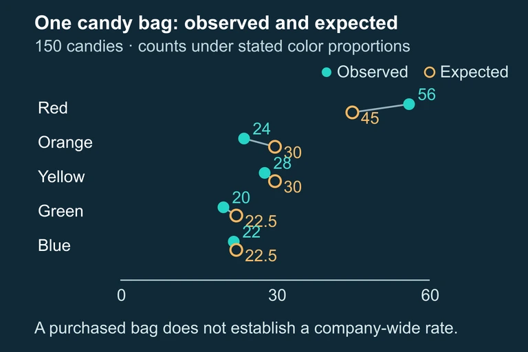
Five observed versus expected candy counts for a 150-candy example. Expected counts include 45,30,30,22.5,22.5. Sampling from one bag does not establish company-wide inference.
Observed color counts from one purchased bag can be compared with the stated model, but this design does not establish company-wide inference.

Question 1 of 5

A researcher claims that customer preferences for 4 flavors are equally distributed. She surveys 200 customers. What are the expected counts for each flavor?

Question 2 of 5

Which of the following is the correct null hypothesis for a chi-square goodness-of-fit test about whether a die is fair?

Question 3 of 5

A goodness-of-fit test has 5 categories. What are the degrees of freedom?

Question 4 of 5

You compute expected counts and find that one category has \(E_i = 3.2\). What should you conclude about the Large Counts condition?

Question 5 of 5

In a goodness-of-fit test with observed counts \(O = \{30, 25, 45\}\) and expected counts \(E = \{33.3, 33.3, 33.3\}\), which category contributes the most to the \(\chi^2\) statistic?