Analyzing Departures
from Linearity
Learn to identify when a linear model fails, interpret residual plots, and recognize nonlinear patterns hiding in your data.
What Is a Linear Model?
A linear model describes the relationship between an explanatory variable \(x\) and a response variable \(y\) with the equation:
A linear model assumes that the true relationship is approximately a straight line. But real data often departs from this assumption: the relationship may be curved, fan-shaped, or contain clusters.
Why Linearity Matters
The Residual Plot: Your Key Tool
A residual is the difference between the observed value and the predicted value:
A residual plot graphs each residual \(e_i\) on the vertical axis against the corresponding \(x_i\) (or \(\hat{y}_i\)) on the horizontal axis. If the linear model is appropriate, the residual plot should show no pattern: just a random scatter of points around the line \(e = 0\).
Good vs. Bad Residual Plots
The LINE Conditions
AP Statistics uses the acronym LINE for the four conditions that must hold for a linear regression model to be valid:
Linearity vs. Equal Variance
Both conditions are checked from the residual plot, but they describe different problems:
| Linearity Violation | Equal Variance Violation | |
|---|---|---|
| Pattern | Curved (U-shape or S-shape) | Fanning (trumpet shape) |
| What fails | The mean of residuals shifts | The spread of residuals changes |
| Residual plot | Points curve above and below \(e = 0\) | Points spread wider on one side |
| Fix | Transform \(x\) or \(y\), or use a nonlinear model | Transform \(y\) (often \(\ln y\)) or use weighted regression |
Recognizing Nonlinear Patterns
How to Analyze Departures
Example 1: Tree Growth
A biologist measures the diameter (cm) and height (m) of 12 trees. She fits the model \(\hat{y} = 2.5 + 0.8x\). Here is the scatterplot with the line:
Example 1: Residual Plot
Now plot the residuals \(e_i = y_i - \hat{y}_i\) against diameter \(x\):
Example 2: Income vs. Spending
An economist fits \(\hat{y} = 200 + 0.6x\) to predict monthly spending \(y\) from income \(x\). Here is the residual plot:
Example 3: Fixing with Transformations
When the residual plot reveals curvature, we can transform the data. Common transformations for AP Statistics:
Can \(r^2\) Tell You About Linearity?
The coefficient of determination \(r^2\) tells you how much variation in \(y\) is explained by the linear model. But a high \(r^2\) does not guarantee linearity.
Common Mistakes
Summary: Residual Plot Patterns
| Pattern | Condition Violated | What to Do |
|---|---|---|
| Random scatter | None: model is appropriate | Proceed with inference |
| U-shape or curve | Linearity | Transform \(x\) or \(y\), or use nonlinear model |
| Fanning (trumpet) | Equal variance | Transform \(y\) (often \(\ln y\)) |
| Groups or clusters | Linearity or lurking variable | Investigate subgroups separately |
| Trend over time | Independence | Use time-series methods |
Worked Example
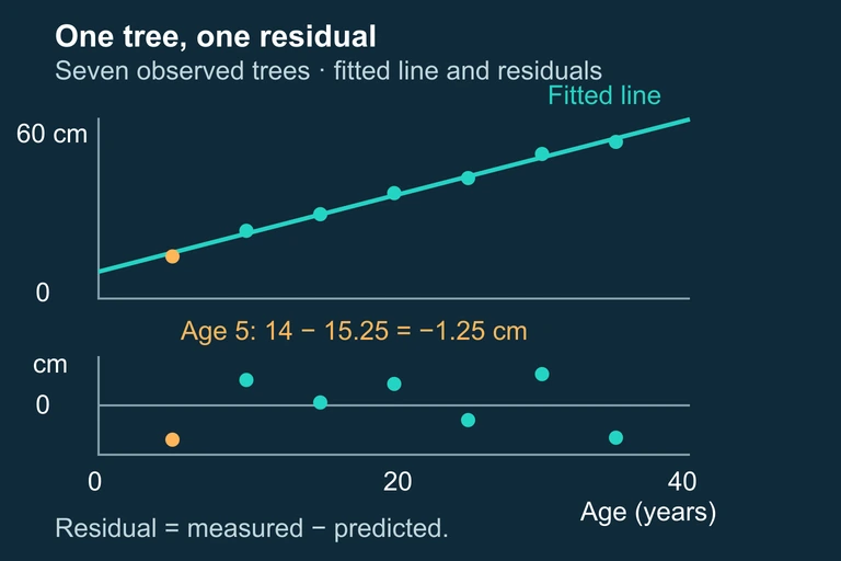
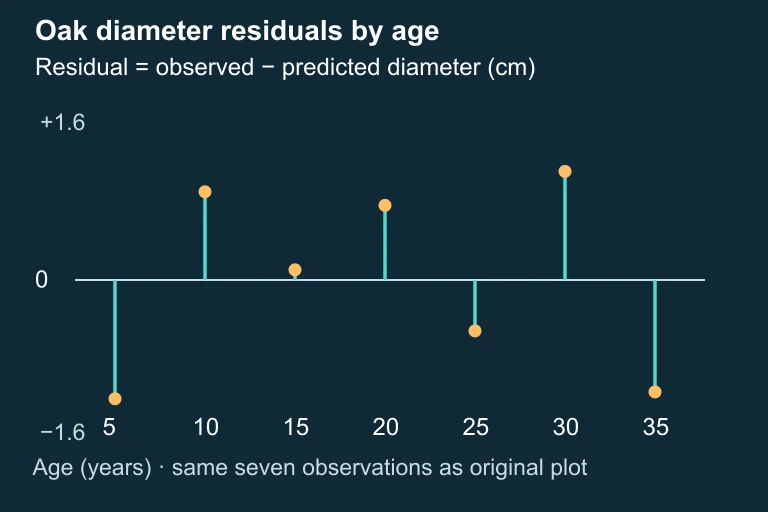
A biologist records age (years) and trunk diameter (centimeters) for seven oak trees. The least-squares line is ŷ = 8.9285714286 + 1.2642857143x, with R² ≈ 0.99463458. The table gives predictions and residuals from that fit. Determine what these data do and do not establish about a linear model. Age (x) | Diameter (y) | Predicted (ŷ) | Residual (e) 5 | 14.0 | 15.250 | −1.250 10 | 22.5 | 21.571 | +0.929 15 | 28.0 | 27.893 | +0.107 20 | 35.0 | 34.214 | +0.786 25 | 40.0 | 40.536 | −0.536 30 | 48.0 | 46.857 | +1.143 35 | 52.0 | 53.179 | −1.179 Analyzing the Oak Tree Residuals Step 1 — Examine r² R² ≈ 0.99463458 means this fitted line accounts for about 99.46% of the observed diameter variation. A high R² alone does not confirm linearity; examine the residuals and the limited sample size. Step 2 — Construct the Residual Plot (mentally or on calculator) At ages 5,10,15,20,25,30,35, the residuals are approximately −1.250,+0.929,+0.107,+0.786,−0.536,+1.143,−1.179 cm. They sum to zero apart from rounding. Both positive and negative residuals occur across the age range; they do not follow a transition from positive values to increasingly negative ones. Step 3 — Identify the Pattern These seven residuals do not establish the previously suggested monotonic curvature. Inspecting their plotted shape is still useful, but the small sample limits conclusions about model form. A high R² and a short residual series cannot certify that the population relationship is exactly linear. No established monotonic curvature; seven points limit the diagnosis. Step 4 — State the Conclusion The fitted line closely summarizes these seven observed pairs. The residuals do not justify rejecting it on the basis of the claimed monotonic pattern or automatically applying a transformation. Continue to check model assumptions and gather more data when prediction matters; high R² alone is not sufficient validation. Retain a provisional linear summary; do not force an unsupported transformation.
Question 1 of 5
A residual plot for a linear regression shows a clear U-shaped pattern. What does this indicate?
Question 2 of 5
A regression of population on year gives \(r^2 = 0.98\), but the residual plot shows strong curvature. Which conclusion is most appropriate?
Question 3 of 5
If the residual plot shows that the spread of residuals increases as \(x\) increases (a fanning pattern), which LINE condition is violated?
Question 4 of 5
A scientist suspects exponential growth in a dataset. She plots \(\ln y\) against \(x\) and the new residual plot shows random scatter. What should she conclude?
Question 5 of 5
Which of the following is the best way to check whether a linear model is appropriate for a dataset?