The Geometric Distribution - AP Statistics

SECTION 1

Historical Context & Motivation

Many real-world situations share a simple but compelling structure: you repeat an experiment under identical conditions until a particular event occurs for the first time. A quality-control inspector tests lightbulbs until one fails, a basketball player shoots free throws until she makes one, or a geneticist breeds organisms until a recessive phenotype appears. The geometric distribution provides the probabilistic framework for all such 'waiting-time' scenarios, formalizing the question: How many trials will it take to get the first success?

The intellectual roots of this distribution lie in the broader development of probability theory during the seventeenth and eighteenth centuries. As mathematicians studied games of chance and actuarial problems, they naturally encountered sequences of independent trials with two possible outcomes—what we now call Bernoulli trials. The geometric distribution emerged as one of the simplest and most elegant consequences of this framework, connecting combinatorial reasoning with the geometric series from which it derives its name.

1654 • The Pascal–Fermat Correspondence

Blaise Pascal and Pierre de Fermat exchange letters on the 'problem of points,' laying the groundwork for formal probability theory and the study of repeated trials.

1713 • Ars Conjectandi Published

Jacob Bernoulli's posthumous masterwork introduces the concept of independent, identically distributed trials (later called Bernoulli trials), the foundation on which the geometric distribution rests.

1837 • Poisson's Systematic Framework

Siméon Denis Poisson publishes work that systematically catalogs discrete distributions, including waiting-time models closely related to the modern geometric distribution.

20th c. • Modern Textbook Formalization

With the rise of mathematical statistics, the geometric distribution is formally defined, its moment-generating function derived, and its memoryless property rigorously proved—securing its place in the standard probability canon.

The central question the geometric distribution addresses is deceptively straightforward: given a fixed probability of success on each trial, what is the probability that the first success occurs on the kth trial? Answering this question rigorously requires only the multiplication rule for independent events and the formula for a geometric series, yet the resulting distribution is remarkably powerful—appearing in quality control, genetics, telecommunications, and game theory alike.

SECTION 2

Core Principles & Definitions

Before working with the geometric distribution, you must verify that the scenario satisfies a specific set of conditions. These conditions mirror those of the binomial setting, with one critical modification: instead of a fixed number of trials, the random variable counts the number of trials required to achieve the first success. If any of the conditions below fails, the geometric model does not apply.

Binary Outcomes

Each trial has exactly two mutually exclusive outcomes: success (the event of interest) and failure. These labels are arbitrary; a 'success' need not be desirable.

Independence

The outcome of any trial does not influence the outcome of any other trial. This independence assumption allows us to multiply probabilities across trials.

Constant Probability

The probability of success, denoted p, remains the same from trial to trial. The probability of failure is q = 1 − p.

Counting to the First Success

The random variable X represents the trial number on which the first success occurs. Thus X can take values 1, 2, 3, … with no upper bound.

Notice how these conditions differ from the binomial setting. In a binomial experiment the number of trials n is fixed in advance and the random variable counts the total number of successes. In the geometric setting, success is guaranteed to happen eventually—we simply do not know when. This subtle shift from 'how many successes in n trials' to 'how many trials until the first success' is the defining hallmark of the geometric distribution.

✦

KEY TAKEAWAY

Think of the geometric distribution like fishing: each cast of your line is an independent trial with the same probability of catching a fish. You keep casting until you land one. The geometric distribution tells you the probability that your first catch comes on the 1st cast, the 2nd cast, the 5th, the 20th, and so on. The 'geometric' name comes from the fact that the probabilities form a geometric sequence—each successive probability is obtained by multiplying the previous one by the constant ratio (1 − p).

SECTION 3

Visual Explanation

The probability distribution of a geometric random variable has a distinctive shape: it starts at its maximum value when X = 1 and decays exponentially as X increases. The following diagram shows the probability mass function (PMF) for a geometric distribution with p = 0.3, illustrating how the probability of achieving the first success on later and later trials diminishes in a characteristic staircase pattern.

The bar chart above displays P(X = k) for k = 1, 2, …, 10 when p = 0.3. Notice how each bar is exactly 0.7 times the height of the previous bar, reflecting the constant ratio (1 − p) = 0.7. The tallest bar occurs at k = 1 because the most probable outcome is succeeding on the very first trial.

Several features are worth observing. First, the distribution is right-skewed—the long tail stretches toward larger values of k, indicating that while most first successes occur relatively early, there is always a nonzero probability of having to wait a very long time. Second, the bars form a geometric sequence with common ratio (1 − p), which is precisely why this is called the geometric distribution. Third, the sum of all bar heights equals 1, confirming that this is a valid probability distribution—a fact guaranteed by the geometric series formula.

A child examines five distinct collectible designs and repeated prizes among opened cereal packages. Collecting all prize types and waiting for the first designated prize use different stopping rules. Define the response variable before generating trials.

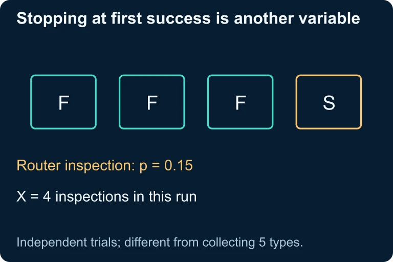Four router trials are labeled failure, failure, failure and success, ending at the first success with p = 0.15. In a separate router example, each independent trial succeeds with probability 0.15. The sequence failure, failure, failure, success gives X = 4, with probability 0.85³ × 0.15. This stopping rule differs from collecting all five cereal-prize types.

SECTION 4

Mathematical Framework

Deriving the probability mass function requires only the multiplication rule for independent events. If the first success occurs on trial k, then the preceding (k − 1) trials must all have been failures and the kth trial must be a success. Since the trials are independent with constant probabilities, we multiply:

PROBABILITY MASS FUNCTION

P(X = k) = (1 − p)^(k−1) × p, k = 1, 2, 3, …

Here p is the probability of success on each trial, k is the trial number on which the first success occurs, and (1 − p) is the probability of failure. The exponent (k − 1) counts the failures before the first success.

We can verify that these probabilities sum to 1 by recognizing the infinite geometric series: Σ (1 − p)^k−1 × p from k = 1 to ∞ equals p × [1 / (1 − (1 − p))] = p × (1/p) = 1. The expected value and variance can be derived using similar series manipulations or moment-generating function techniques.

EXPECTED VALUE (MEAN)

μ_X = E(X) = 1/p

The mean tells you the average number of trials needed to get the first success. For example, if p = 0.2 (a 20% chance each trial), you expect on average 1/0.2 = 5 trials.

VARIANCE AND STANDARD DEVIATION

σ²_X = (1 − p) / p² σ_X = √[(1 − p) / p²]

The variance measures how spread out the waiting times are. As p decreases, both the mean and the variance increase—low-probability events require more trials on average and exhibit greater variability in timing.

A particularly useful formula for AP Statistics involves cumulative probabilities. The probability that the first success occurs on or before trial k (equivalently, the probability that you need at most k trials) is given by:

CUMULATIVE PROBABILITY

P(X ≤ k) = 1 − (1 − p)^k

This formula is derived from the complement rule: P(X ≤ k) = 1 − P(X > k). The event X > k means all k trials were failures, which has probability (1 − p)^k. This shortcut avoids the need to sum individual PMF values.

SECTION 5

Key Properties & the Memoryless Property

The geometric distribution possesses a remarkable and unique property among discrete distributions: the memoryless property. In precise terms, if X is geometric, then P(X > s + t | X > s) = P(X > t) for all positive integers s and t. Intuitively, this means that if you have already failed on the first s trials, the probability of needing at least t more trials is the same as if you were starting fresh. The past failures give you no information about how much longer you will have to wait. The geometric distribution is the only discrete distribution with this property.

The four-panel summary above organizes the essential formulas and properties of the geometric distribution. The PMF and CDF formulas (left and right) are the computational workhorses, while the mean/variance formulas and the memoryless property provide deeper insight into the distribution's behavior.

On the AP Statistics exam, the memoryless property is occasionally tested directly, but more frequently it appears implicitly in questions that ask for conditional probabilities. For instance, 'Given that a basketball player has missed his first three free throws, what is the probability he will need more than two additional attempts to make one?' If the geometric conditions hold, the answer is simply P(X > 2) = (1 − p)², computed as though the first three misses never happened.

💡

AP EXAM TIP

When determining P(X > k) for a geometric random variable, use the shortcut (1 − p)^k rather than summing individual PMF values. This is faster and less error-prone on both the multiple-choice and free-response sections.

SECTION 6

Worked Example

A consumer electronics company knows from historical data that 15% of its wireless routers fail the final quality inspection. An inspector tests routers one at a time, and we define 'success' as finding a defective router. We want to answer several questions about this geometric setting.

Quality Inspection — Geometric Distribution

1
Step 1 — Verify the Geometric Conditions

Each inspection has two outcomes (defective or not), inspections are independent of one another, the probability of finding a defective router is constant at p = 0.15, and the inspector continues until the first defective router is found. All four conditions are satisfied, so X ~ Geometric(p = 0.15).
2
Step 2 — Find P(X = 4)

We want the probability that the first defective router is found on the 4th inspection. Using the PMF: P(X = 4) = (1 − 0.15)³ × 0.15 = (0.85)³ × 0.15 = 0.614125 × 0.15.

P(X = 4) ≈ 0.0921
3
Step 3 — Find P(X ≤ 5)

We want the probability that the first defective router is found within the first 5 inspections. Using the CDF shortcut: P(X ≤ 5) = 1 − (1 − 0.15)⁵ = 1 − (0.85)⁵ = 1 − 0.4437 ≈ 0.5563.

P(X ≤ 5) ≈ 0.5563
4
Step 4 — Find the Expected Value and Standard Deviation

The mean number of inspections until finding the first defective router is μ = 1/p = 1/0.15 ≈ 6.667. The standard deviation is σ = √[(1 − p)/p²] = √[0.85/0.0225] = √37.778 ≈ 6.147. The large standard deviation relative to the mean reflects the heavy right skew of the distribution.

μ ≈ 6.67 inspections, σ ≈ 6.15 inspections
5
Step 5 — Interpret in Context

On average, the inspector must test about 6 or 7 routers before finding the first defective one. There is roughly a 55.6% chance that a defective router will appear within the first 5 tests, and about a 9.2% chance that the 4th router tested is the first defective one. The relatively large standard deviation tells us that the actual number of inspections can vary substantially from the mean.

SECTION 7

Geometric vs. Binomial: Strengths & Limitations

Students often confuse the geometric and binomial distributions because both arise from independent Bernoulli trials with constant probability p. The critical distinction lies in what is fixed and what is random. Understanding this comparison is essential for the AP exam, where you must identify the correct distribution before performing any calculation.

Feature	Binomial Distribution	Geometric Distribution
What is fixed?	Number of trials n	Nothing—trials continue until first success
Random variable counts	Number of successes in n trials	Number of trials until first success
Possible values	0, 1, 2, …, n (finite)	1, 2, 3, … (infinite)
Mean	np	1/p
Variance	np(1 − p)	(1 − p)/p²
Shape	Approximately symmetric when np ≥ 10 and n(1−p) ≥ 10	Always right-skewed
Memoryless?	No	Yes

Side-by-side comparison of the binomial and geometric distributions

✦

KEY TAKEAWAY

When deciding between the binomial and geometric distributions on the AP exam, ask one question: Is the number of trials determined in advance? If yes, use binomial. If the process continues until a certain outcome occurs for the first time, use geometric. This single diagnostic question resolves the vast majority of identification problems.

It is also important to recognize the limitations of the geometric model. In practice, trials may not be perfectly independent (for example, a student's confidence may change after several failures), or the probability may shift over time (a machine's defect rate may increase as it wears). When these violations are mild, the geometric distribution remains a useful approximation; when they are severe, more sophisticated models such as the negative binomial or Markov-chain-based waiting-time distributions may be required.

SECTION 8

Connection to Advanced Theory

The geometric distribution is the simplest case of a broader family of distributions that model waiting times in sequences of Bernoulli trials. Understanding how it fits into this larger framework will deepen your understanding and prepare you for topics beyond the AP exam.

Feature	Geometric Distribution	Negative Binomial Distribution
What it counts	Trials until the 1st success	Trials until the rth success
Parameters	p only	r and p
Mean	1/p	r/p
Relationship	Special case where r = 1	Sum of r independent Geometric(p) random variables
Memoryless?	Yes	No (for r > 1)

The geometric distribution as a special case of the negative binomial

There is also a continuous analogue: the exponential distribution models the waiting time until the first event in a continuous-time Poisson process, and it too is memoryless. Just as the geometric distribution is the only discrete memoryless distribution, the exponential distribution is the only continuous memoryless distribution. If you continue into college probability courses, you will see that these two distributions are deeply connected through the relationship between discrete and continuous stochastic processes.

ℹ

LOOKING AHEAD

Although the negative binomial and exponential distributions are beyond the scope of the AP Statistics exam, understanding that the geometric distribution is the simplest 'waiting-time' distribution will give you an intuitive foundation for these more general models. On the AP exam, you should be able to recognize geometric settings, apply the PMF, calculate cumulative probabilities using the complement shortcut, and compute the mean and standard deviation.

SECTION 9

Practice Problems

Question 1: CONCEPTUAL

Which of the following scenarios can be modeled by a geometric distribution?

A. Counting the number of heads in 20 flips of a fair coin
B. Counting how many times a six-sided die is rolled until a 3 appears for the first time
C. Recording the heights of 50 randomly selected students
D. Counting the total number of defective items in a shipment of 500
E. Drawing cards from a deck without replacement until an ace is drawn

Show answer (B)

The correct answer is B. Rolling a die until a 3 appears satisfies all geometric conditions: binary outcomes (3 or not-3), independent trials, constant probability p = 1/6, and counting trials to the first success. Option A is binomial (fixed n = 20, counting total successes). Option C involves a continuous measurement, not a count of trials. Option D is binomial (fixed n = 500, counting successes). Option E violates independence because cards are drawn without replacement, changing the probability on each draw.

Question 2: BASIC CALCULATION

A certain type of seed has a 0.40 probability of germinating. Seeds are planted one at a time in separate pots. What is the probability that the first seed to germinate is the third one planted?

A. 0.064
B. 0.096
C. 0.144
D. 0.216
E. 0.360

Show answer (C)

The correct answer is C. Using the geometric PMF with p = 0.40 and k = 3: P(X = 3) = (1 − 0.40)²(0.40) = (0.60)²(0.40) = 0.36 × 0.40 = 0.144. Option A (0.064) equals (0.40)³, which incorrectly treats three successes rather than two failures then a success. Option B (0.096) equals (0.60)(0.40)², confusing the order of failures and successes. Option D (0.216) equals (0.60)³, the probability of three consecutive failures. Option E (0.360) equals (0.60)(0.60) without the final success factor.

Question 3: INTERMEDIATE

A spinner has a 25% chance of landing on blue on any given spin. Spins are independent. What is the probability that the first blue result occurs on or before the 5th spin?

A. 0.2373
B. 0.6328
C. 0.7627
D. 0.7500
E. 0.9990

Show answer (C)

The correct answer is C. Using the cumulative probability formula: P(X ≤ 5) = 1 − (1 − 0.25)⁵ = 1 − (0.75)⁵ = 1 − 0.2373 ≈ 0.7627. Option A (0.2373) is actually P(X > 5) = (0.75)⁵, the probability that blue does NOT appear in the first 5 spins—the complement of the correct answer. Option B (0.6328) does not correspond to any standard geometric calculation for these parameters. Option D (0.7500) appears to be 3/4 or simply 1 − p, which does not apply here. Option E (0.9990) is far too high for only 5 trials with p = 0.25.

Question 4: APPLIED

4 pts

A pharmaceutical company is screening chemical compounds to find one that effectively inhibits a certain enzyme. Based on prior research, each compound tested independently has a 0.05 probability of being effective. The company tests compounds one at a time. (a) What is the expected number of compounds the company must test to find the first effective one? (b) What is the standard deviation of the number of compounds tested? (c) What is the probability that the company finds an effective compound within the first 10 tests? (d) Interpret the result of part (c) in the context of the problem.

Show answer

RUBRIC (4 points): Point 1 (Expected Value): μ = 1/p = 1/0.05 = 20 compounds. The company should expect to test 20 compounds on average before finding the first effective one. Point 2 (Standard Deviation): σ = √[(1 − p)/p²] = √[0.95/0.0025] = √380 ≈ 19.49 compounds. The large standard deviation (nearly as large as the mean) reflects the heavy right skew of the geometric distribution when p is small. Point 3 (Cumulative Probability Calculation): P(X ≤ 10) = 1 − (1 − 0.05)¹⁰ = 1 − (0.95)¹⁰ = 1 − 0.5987 ≈ 0.4013. Point 4 (Interpretation in Context): There is approximately a 40.1% probability that the company will find an effective compound within the first 10 tests. This means that even after testing 10 compounds, there is a roughly 60% chance that the company has not yet found an effective one, which underscores the challenge and cost of drug screening when the per-trial success rate is only 5%.

Question 5: CRITICAL THINKING

4 pts

A basketball player makes free throws with probability p = 0.80. She steps to the free-throw line and misses her first three attempts. Her coach claims that she is 'due' to make the next one because she has missed so many in a row. (a) State the assumptions required for the geometric model to apply to this situation. (b) Using the memoryless property, explain whether the coach's reasoning is statistically valid. (c) Calculate P(X > 5 | X > 3), where X is the number of the trial on which the first made free throw occurs. Show your work using both the memoryless property and the conditional probability formula to verify they give the same result. (d) Discuss a real-world reason why the geometric model might NOT perfectly apply to free-throw shooting, and explain how this could affect the validity of using the memoryless property.

Show answer

RUBRIC (4 points): Point 1 (Assumptions): For the geometric model: (1) Each free throw has exactly two outcomes (make or miss), (2) free throws are independent of one another, (3) the probability of making each free throw is constant at p = 0.80, and (4) the random variable X counts the trial number on which the first made free throw occurs. Point 2 (Memoryless Property Explanation): The coach's reasoning is a form of the gambler's fallacy and is NOT statistically valid under the geometric model. The memoryless property states P(X > s + t | X > s) = P(X > t). Given that she has already missed 3 shots, her probability of making the next shot is still exactly p = 0.80—the same as it was before any shots were taken. The three consecutive misses provide no information about the outcome of future shots. Point 3 (Calculation): Using the memoryless property: P(X > 5 | X > 3) = P(X > 2) = (1 − 0.80)² = (0.20)² = 0.04. Verification using the conditional probability formula: P(X > 5 | X > 3) = P(X > 5 AND X > 3)/P(X > 3) = P(X > 5)/P(X > 3) = (0.20)⁵/(0.20)³ = 0.00032/0.008 = 0.04. Both methods yield 0.04, confirming the memoryless property. Point 4 (Real-World Discussion): In reality, free-throw shooting may not satisfy the independence or constant-probability assumptions. Psychological factors such as frustration after consecutive misses (or increased focus) could alter p from shot to shot. Physical fatigue during a game could also change the probability over time. If p is not truly constant—for example, if it decreases after misses due to loss of confidence—then the memoryless property does not hold, and the probability of continuing to miss could be higher (or lower) than the geometric model predicts. This would make the geometric distribution an imperfect model for actual free-throw sequences.

SUMMARY

Summary

The geometric distribution models the number of independent Bernoulli trials needed to achieve the first success, where each trial has a constant probability of success p. Its probability mass function is P(X = k) = (1 − p)^k−1 × p for k = 1, 2, 3, …, producing a right-skewed distribution whose probabilities decay by the constant factor (1 − p) at each step.

The expected value is μ = 1/p and the variance is σ² = (1 − p)/p². The cumulative probability shortcut P(X ≤ k) = 1 − (1 − p)^k eliminates the need to sum individual PMF values. The memoryless property—unique among discrete distributions—states that past failures do not change future probabilities: P(X > s + t | X > s) = P(X > t). For the AP exam, be sure to distinguish the geometric distribution from the binomial distribution by asking whether the number of trials is fixed in advance (binomial) or determined by when the first success occurs (geometric).