The Central Limit Theorem - AP Statistics

SECTION 1

Historical Context & Motivation

The Central Limit Theorem (CLT) stands as one of the most profound results in all of probability and statistics, providing the theoretical foundation for virtually every confidence interval and hypothesis test you will encounter on the AP Statistics exam. The theorem answers a deceptively simple question: if you repeatedly draw random samples from any population and compute their means, what shape will the distribution of those means take? Before the CLT was formalized, mathematicians had noticed that averages of measurements—even from wildly skewed or irregular distributions—seemed to cluster around the population mean in a bell-shaped pattern. The quest to understand and prove this empirical observation spanned more than two centuries of mathematical development.

1733 • De Moivre's Approximation

Abraham de Moivre demonstrated that the binomial distribution approaches a bell curve as the number of trials grows, establishing the first special case of the CLT for coin-flipping experiments.

1812 • Laplace's Generalization

Pierre-Simon Laplace extended De Moivre's result, proving that the sum of a large number of independent random variables—regardless of their individual distributions—tends toward a normal distribution. This was the first broadly general statement of the theorem.

1901 • Lyapunov's Rigorous Proof

Aleksandr Lyapunov used characteristic functions to provide the first fully rigorous proof of the CLT under general conditions, establishing the mathematical standard that would anchor modern probability theory.

1920s • Lindeberg–Lévy Refinement

Jarl Waldemar Lindeberg and Paul Lévy established precise necessary and sufficient conditions for the CLT, clarifying when the theorem holds even for non-identically distributed random variables.

The central question that drove this entire line of inquiry was both practical and elegant: Why does the normal distribution appear so pervasively in real-world data? Heights, test scores, measurement errors, and countless other phenomena are approximately normal—not because nature prefers bell curves, but because many observed quantities are effectively averages or sums of many small, independent influences. The CLT explains this universality and, critically for AP Statistics, it justifies using normal-based inference procedures even when the underlying population is not normally distributed.

SECTION 2

Core Principles & Definitions

Before stating the theorem formally, it is essential to distinguish between two related but distinct concepts. A population distribution describes the values of every individual in the population—it can be any shape at all: skewed, bimodal, uniform, or already normal. A sampling distribution describes the behavior of a statistic (such as the sample mean x̄) computed across all possible random samples of a fixed size n. The CLT speaks exclusively about this second distribution—the sampling distribution of x̄—and asserts that it becomes approximately normal for sufficiently large n, regardless of the population's shape.

Shape Convergence

As sample size n increases, the sampling distribution of x̄ approaches a normal distribution, regardless of the population's shape.

Center Preservation

The mean of the sampling distribution equals the population mean: μ_x̄ = μ. The sample mean is an unbiased estimator of the population mean.

Spread Reduction

The standard deviation of x̄ is σ / √n, which shrinks as the sample size grows. Larger samples produce more precise estimates.

Independence Requirement

Observations must be independent. For sampling without replacement, the population must be at least 10 times the sample size (the 10% condition).

Sample Size Threshold

The common AP guideline is n ≥ 30 for most populations. More skewed populations require larger n; populations that are already normal require any n.

✦

KEY TAKEAWAY

Think of the CLT like a smoothie blender. Each fruit you toss in—strawberry, banana, kiwi—has a very different shape and texture (analogous to differently shaped population distributions). But once you blend many pieces together, you always get the same smooth consistency. Similarly, when you average together many independent observations, the resulting distribution of that average always smooths out into the same recognizable bell curve. The more observations you blend (larger n), the smoother the result.

SECTION 3

Visual Explanation

The most powerful way to internalize the CLT is to watch it in action. The diagram below shows three different population distributions—a strongly right-skewed exponential, a uniform, and a bimodal distribution—alongside the sampling distributions of x̄ that emerge at sample sizes n = 2, n = 10, and n = 30. Notice how even the most irregular population shape yields a nearly perfect bell curve by n = 30.

Each row shows a different population shape (left column). Moving right, the sampling distribution of x̄ becomes progressively more bell-shaped as n increases from 2 to 10 to 30, illustrating the CLT's shape convergence regardless of the original population distribution.

Several features of the diagram are worth emphasizing. In the top row, the exponential population is heavily right-skewed, yet by n = 30 the sampling distribution of x̄ is nearly symmetric. The uniform population (middle row) converges even faster—a triangular shape appears by n = 2, and near-normality is reached around n = 10. The bimodal population (bottom row) is the most stubborn, retaining a slight flattening at small sample sizes, but it too yields a convincing bell curve by n = 30. This visual pattern is exactly what the AP exam expects you to understand: the more the population departs from normality, the larger the sample size needed for the CLT to produce a good approximation.

A filling line loads bottles into trays while one statistic is recorded for each tray. A tray contains individual observations, but its average contributes one value to a distribution of sample means. Repeating the sampling process reveals how that statistic varies.

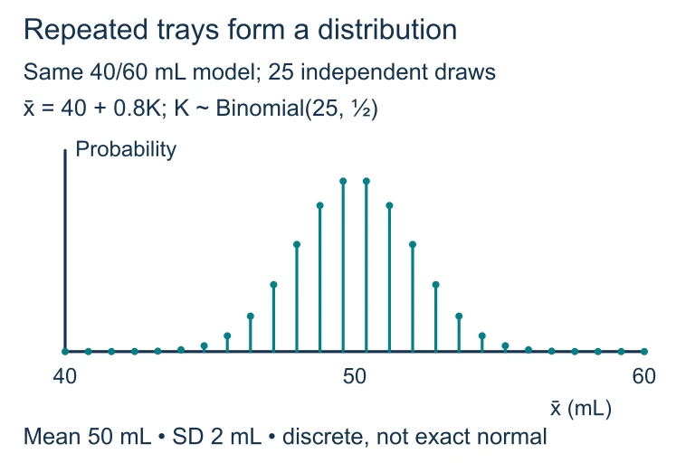Twenty-six possible sample means appear as discrete probability bars with a normal approximation drawn for comparison. For 25 independent fills equally likely to be 40 or 60 mL, K is binomial with n = 25 and p = 0.5, and the tray mean is 40 + 0.8K. The exact distribution is discrete, centered at 50 mL with standard deviation 2 mL. A normal curve approximates its shape.

SECTION 4

Mathematical Framework

The CLT can be stated concisely using formal notation. Let X₁, X₂, …, Xₙ be independent random variables drawn from a population with mean μ and finite standard deviation σ. Define the sample mean as x̄ = (X₁ + X₂ + … + Xₙ) / n. Then as n → ∞, the standardized variable Z = (x̄ − μ) / (σ / √n) converges in distribution to the standard normal N(0, 1). For practical purposes on the AP exam, you need the following equations.

MEAN OF THE SAMPLING DISTRIBUTION

μ_x̄ = μ

The mean of the sampling distribution of x̄ equals the population mean μ. This holds for any sample size, not just large ones, and is why x̄ is called an unbiased estimator.

STANDARD DEVIATION OF THE SAMPLING DISTRIBUTION

σ_x̄ = σ / √n

Often called the standard error of the mean. As n increases, σ_x̄ decreases by a factor of √n, meaning quadrupling the sample size halves the standard error.

CLT APPROXIMATION

x̄ ~ N(μ, σ / √n) when n is sufficiently large

This is the complete CLT statement: the sampling distribution of x̄ is approximately normal with center μ and spread σ / √n. On the AP exam, 'sufficiently large' typically means n ≥ 30 unless the population is already normal.

STANDARDIZATION (Z-SCORE FOR x̄)

z = (x̄ − μ) / (σ / √n)

This z-score measures how many standard errors a particular sample mean x̄ falls from the population mean μ. Use this to find probabilities involving x̄ from the standard normal table or your calculator's normalcdf function.

💡

AP Exam Tip

When the population is already normal, the sampling distribution of x̄ is exactly normal for any sample size n—no minimum n is required. The n ≥ 30 guideline only applies when the population is non-normal. For moderately skewed populations, n ≥ 15 may suffice. Always check the problem's context.

SECTION 5

Conditions & Sample Size Guidelines

Applying the CLT correctly on the AP exam requires you to verify specific conditions before concluding that the sampling distribution is approximately normal. Free-response graders look for explicit statements of these conditions, so understanding them in detail is essential for earning full credit.

A decision flowchart for determining when the CLT applies. Start at the top: verify independence first, then assess normality. If the population is already normal, any sample size works. Otherwise, the required n depends on the degree of skewness.

Population Shape	Minimum n for CLT	Reasoning
Normal	Any n	x̄ is exactly normal when the population is normal
Symmetric, non-normal (e.g., uniform)	n ≥ 15	Symmetry means convergence is rapid
Moderately skewed	n ≥ 30	The standard AP guideline for most non-normal populations
Heavily skewed or outlier-prone	n ≥ 40–50+	Extreme skew (e.g., income data) needs larger samples

Sample size guidelines for CLT approximation by population shape

⚠

The 10% Condition

When sampling without replacement from a finite population, the sampled values are technically not independent. However, if the sample size n is no more than 10% of the population size N (i.e., n ≤ 0.10N), the dependence is negligible and we treat observations as independent. On AP free-response questions, always state this condition explicitly when verifying the CLT.

SECTION 6

Worked Example

A bottling machine fills soda cans with a mean fill volume of μ = 355 mL and a standard deviation of σ = 4 mL. The distribution of individual fill volumes is right-skewed. A quality control inspector selects a random sample of 50 cans. What is the probability that the sample mean fill volume is less than 354 mL?

Finding P(x̄ < 354) Using the CLT

1
Step 1 — Check Conditions

Independence: The 50 cans are randomly selected, and 50 is certainly less than 10% of all cans the machine produces (tens of thousands daily), so the independence condition is satisfied. Normality: Although the population is right-skewed, n = 50 ≥ 30, so by the CLT the sampling distribution of x̄ is approximately normal.
2
Step 2 — Identify Parameters of the Sampling Distribution

μ_x̄ = μ = 355 mL. The standard error is σ_x̄ = σ / √n = 4 / √50 = 4 / 7.071.

σ_x̄ ≈ 0.5657 mL
3
Step 3 — Compute the z-Score

z = (x̄ − μ) / (σ / √n) = (354 − 355) / 0.5657 = −1 / 0.5657.

z ≈ −1.768
4
Step 4 — Find the Probability

Using the standard normal table or calculator: P(Z < −1.768). On a TI-84, enter normalcdf(−1E99, −1.768, 0, 1).

P(x̄ < 354) ≈ 0.0385
5
Step 5 — Interpret in Context

There is approximately a 3.85% probability that a random sample of 50 cans will have a mean fill volume below 354 mL. This is a relatively unlikely outcome if the machine is operating correctly, which is why quality control inspectors might flag such a result as evidence of under-filling.

SECTION 7

Strengths, Limitations & Common Misconceptions

Strengths	Limitations
Applies regardless of population shape, making normal-based inference widely usable	Requires a sufficiently large n; for heavily skewed populations, n = 30 may not be enough
Provides a simple, closed-form approximation (normal distribution) rather than requiring simulation	Assumes finite variance; fails for distributions with infinite variance (e.g., Cauchy)
Underpins z-tests, t-tests, confidence intervals, and regression inference	Approximation quality is hard to gauge exactly without simulation or Berry–Esseen bounds
Sample means become more precise as n grows (σ_x̄ → 0)	Does not apply to statistics other than means/sums without additional justification

Strengths and limitations of the Central Limit Theorem

Common Misconceptions on the AP Exam

"The CLT says the data become normal." Incorrect. The individual data values retain the population's shape. The CLT applies only to the sampling distribution of the sample mean (or sum), not to individual observations.
"n ≥ 30 is always required." Incorrect. If the population is already approximately normal, any sample size is sufficient. The n ≥ 30 rule is a guideline for non-normal populations.
"The CLT applies to any statistic." Not automatically. The CLT specifically addresses means and sums. While the sampling distribution of a proportion is also approximately normal (by a related argument), statistics like the median or range require different theory.
"The standard deviation of x̄ is σ." The standard deviation of x̄ is σ / √n, not σ. Forgetting the √n in the denominator is one of the most common calculation errors.

✦

KEY TAKEAWAY

The CLT is a statement about the shape of the sampling distribution, not the shape of the data. Imagine you are a pollster summarizing opinions: one individual response might be extreme, but the average of 1,000 responses is remarkably stable and predictable. The CLT guarantees that this 'averaging effect' produces a normal sampling distribution, which is why we can use z-scores and normal tables to make probabilistic statements about sample means.

SECTION 8

Connection to Inference & Advanced Theory

The CLT is not merely an abstract theorem—it is the engine that powers the inferential procedures you use throughout the AP Statistics course. Every time you construct a confidence interval for a mean or conduct a hypothesis test about a mean, you are implicitly relying on the CLT's guarantee that x̄ is approximately normally distributed. The table below highlights how the CLT connects to its more advanced counterpart when the population standard deviation σ is unknown.

Feature	CLT with Known σ (z-procedures)	Unknown σ (t-procedures)
Standard error formula	σ / √n (population σ known)	s / √n (sample s replaces σ)
Reference distribution	Standard normal N(0, 1)	t-distribution with df = n − 1
Tails	Thinner tails	Heavier tails (more conservative)
Convergence as n → ∞	Already N(0, 1)	t → N(0, 1) as df → ∞
Typical AP exam usage	Rarely tested (σ seldom known in practice)	Primary tool for inference about means

Comparison of z-based and t-based inference for means

Beyond the AP curriculum, the CLT extends in several powerful directions. The multivariate CLT shows that vectors of sample means converge to a multivariate normal distribution, which underpins multiple regression theory. The Berry–Esseen theorem quantifies the rate of convergence, giving an upper bound on the approximation error that decreases at rate 1/√n. In Bayesian statistics, the CLT justifies the use of normal approximations to posterior distributions in large samples. These extensions illustrate that the CLT is not merely a stepping stone—it is a central pillar of statistical theory at every level.

SECTION 9

Practice Problems

Question 1: CONCEPTUAL

A population of household incomes is strongly right-skewed. A researcher takes a simple random sample of 100 households and computes the sample mean income x̄. Which of the following best describes the sampling distribution of x̄?

A. It is strongly right-skewed because the population is strongly right-skewed.
B. It is approximately normal with mean μ and standard deviation σ.
C. It is approximately normal with mean μ and standard deviation σ / √100.
D. It is exactly normal with mean μ and standard deviation σ / √100.
E. The shape cannot be determined without knowing the exact population distribution.

Show answer (C)

C is correct. By the Central Limit Theorem, with n = 100 (well above 30), the sampling distribution of x̄ is approximately normal regardless of the population's skewness. The mean of the sampling distribution is μ, and its standard deviation is σ / √n = σ / √100 = σ / 10. Choice A is wrong because the CLT tells us the sampling distribution becomes approximately normal for large n, even if the population is skewed. Choice B is wrong because it states the standard deviation as σ rather than σ / √n—this describes the population, not the sampling distribution of x̄. Choice D is wrong because the sampling distribution is only approximately (not exactly) normal when the population is non-normal. Choice E is wrong because the CLT's power is precisely that we can determine the approximate shape without knowing the exact population distribution.

Question 2: BASIC CALCULATION

The weights of packages shipped by a company have a mean of 12 pounds and a standard deviation of 3 pounds. If a random sample of 36 packages is selected, what is the standard deviation of the sampling distribution of x̄?

A. 0.083 pounds
B. 0.25 pounds
C. 0.50 pounds
D. 2.00 pounds
E. 3.00 pounds

Show answer (C)

C is correct. The standard deviation of the sampling distribution (standard error) is σ_x̄ = σ / √n = 3 / √36 = 3 / 6 = 0.50 pounds. Choice A (0.083) would result from dividing σ by n instead of √n (i.e., 3/36), which is a common error. Choice B (0.25) would result from dividing σ by n and rounding incorrectly or dividing by 12 instead of 6. Choice D (2.00) results from subtracting 1 from σ rather than dividing by √n. Choice E (3.00) represents the population standard deviation σ, not the standard error of x̄.

Question 3: INTERMEDIATE

Commute times for workers in a large city have a mean of 38 minutes and a standard deviation of 12 minutes. The distribution is right-skewed. A transit planner takes a random sample of 64 workers. What is the probability that the sample mean commute time exceeds 40 minutes?

A. 0.0082
B. 0.0446
C. 0.0918
D. 0.4338
E. 0.5662

Show answer (C)

C is correct. First, since n = 64 ≥ 30 and we have a random sample, the CLT applies. The standard error is σ_x̄ = 12 / √64 = 12 / 8 = 1.5 minutes. The z-score is z = (40 − 38) / 1.5 = 2 / 1.5 ≈ 1.333. Using the standard normal table, P(Z > 1.333) ≈ 1 − 0.9082 = 0.0918. Choice A (0.0082) corresponds to approximately z = 2.40, which would result from using σ = 12 directly without dividing by √n. Choice B (0.0446) corresponds to approximately z = 1.70, a miscalculation. Choice D (0.4338) corresponds to z ≈ 0.167, as if the standard error were 12 instead of 1.5. Choice E (0.5662) equals 1 − 0.4338, the complementary error of the same mistake.

Question 4: APPLIED

4 pts

A pharmaceutical company tests the dissolution time of a new tablet formulation. From extensive testing, the dissolution time has a mean of μ = 22 minutes and a standard deviation of σ = 5 minutes. The distribution is moderately right-skewed. A quality analyst randomly selects 40 tablets from a large production batch. (a) Describe the sampling distribution of the sample mean dissolution time x̄. Justify your answer by verifying the appropriate conditions. (b) The company's specification requires that the mean dissolution time for a batch be between 20.5 and 23.5 minutes. Find the probability that the sample mean falls within this specification range. (c) Suppose the analyst could only sample 10 tablets instead. Explain why it would or would not be appropriate to use the normal model for the sampling distribution of x̄ in this case.

Show answer

Part (a) — 2 points: E (1 point): Independence: The 40 tablets are randomly selected and 40 is less than 10% of the large production batch, so the independence condition is met. Normality: The population is moderately right-skewed, but n = 40 ≥ 30, so by the Central Limit Theorem the sampling distribution of x̄ is approximately normal. P (1 point): The sampling distribution of x̄ is approximately N(22, 5/√40) = N(22, 0.7906). That is, approximately normal with mean 22 minutes and standard deviation 0.7906 minutes. Part (b) — 1 point: z₁ = (20.5 − 22) / 0.7906 = −1.5/0.7906 ≈ −1.897. z₂ = (23.5 − 22) / 0.7906 = 1.5/0.7906 ≈ 1.897. P(−1.897 < Z < 1.897) = P(Z < 1.897) − P(Z < −1.897) ≈ 0.9712 − 0.0288 = 0.9424. There is approximately a 94.2% probability that the sample mean falls within the specification range. Part (c) — 1 point: With n = 10, the sample size is less than 30, and the population is described as moderately right-skewed. The CLT does not guarantee approximate normality for such a small sample from a skewed population. Therefore, it would NOT be appropriate to use the normal model for the sampling distribution of x̄ with n = 10. A larger sample or evidence that the population is closer to normal would be needed.

Question 5: CRITICAL THINKING

4 pts

A statistics student claims: "If I take a large enough sample, I can always use the Central Limit Theorem, so conditions like random sampling and independence don't matter." Evaluate this claim by addressing each of the following: (a) Explain why the independence/randomness condition cannot be bypassed simply by increasing sample size. Provide a specific example of how violating this condition leads to incorrect conclusions. (b) A certain population has a distribution that follows a Cauchy distribution (a symmetric, bell-shaped distribution with extremely heavy tails and no finite mean or variance). Explain whether the CLT applies to samples drawn from this population and why. (c) Consider two populations: Population A is uniform on [0, 10] and Population B is exponential with mean 5. For a sample of size n = 25, which population's sampling distribution of x̄ would be better approximated by a normal distribution? Justify your reasoning using properties of the CLT.

Show answer

Part (a) — 2 points: Point 1: The student's claim is incorrect. The CLT requires that observations be independent (or approximately independent via the 10% condition). Increasing sample size does not fix dependence; it can actually amplify bias. Point 2: Example: Suppose a researcher surveys 10,000 people, but all respondents are from a voluntary online poll (not a random sample). The sample mean will systematically over- or under-represent certain groups (selection bias). No matter how large the sample, the sampling distribution of x̄ will be centered on the biased mean rather than the true population mean μ. The CLT governs the shape of the sampling distribution, but it cannot correct for bias introduced by non-random sampling. Part (b) — 1 point: The CLT does NOT apply to the Cauchy distribution because the Cauchy distribution has no finite mean and no finite variance. A fundamental requirement of the CLT is that the population must have a finite variance σ². Without this condition, the standard error σ/√n is undefined, and the sampling distribution of x̄ from a Cauchy population remains Cauchy regardless of sample size—it never converges to normality. This is a classic counterexample demonstrating that the CLT has mathematical preconditions that cannot be ignored. Part (c) — 1 point: Population A (uniform) would be better approximated by a normal distribution at n = 25. The uniform distribution is perfectly symmetric, so the CLT produces a good normal approximation even at relatively small sample sizes (n ≥ 15 is typically sufficient). Population B (exponential) is strongly right-skewed, meaning convergence to normality is slower and typically requires n ≥ 30 or more. At n = 25, the sampling distribution from the exponential population would still exhibit some right skewness, whereas the sampling distribution from the uniform population would be nearly perfectly normal. The key principle is that the rate of convergence depends on how far the population departs from normality—symmetric distributions converge fastest.

SUMMARY

Summary

The Central Limit Theorem states that the sampling distribution of the sample mean x̄ is approximately normal for sufficiently large sample sizes, regardless of the population's shape. The center of this distribution is the population mean μ, and its spread is measured by the standard error σ / √n, which decreases as the sample size grows. Before applying the CLT on the AP exam, you must verify two conditions: independence (random sampling and the 10% condition) and sample size adequacy (generally n ≥ 30 for non-normal populations, though symmetric populations converge faster and normal populations need no minimum n).

The CLT is the theoretical backbone of confidence intervals and hypothesis tests for means. Remember: the theorem describes the behavior of sample means, not individual data values. The z-score formula z = (x̄ − μ) / (σ / √n) converts any sample mean to the standard normal scale, enabling probability calculations. Master the conditions, the formulas, and the interpretation, and you will be well-prepared for any CLT question on the AP Statistics exam.