Summary Statistics for a Quantitative Variable - AP Statistics

SECTION 1

Historical Context & Motivation

Long before the formal discipline of statistics existed, scholars and administrators grappled with a fundamental challenge: how to distill large collections of numerical observations into compact, meaningful descriptions. Census records from ancient civilizations already demanded some notion of a typical value — a single number that could stand in for an entire population. The intellectual journey from ad hoc averaging to a rigorous framework of summary statistics spans centuries of mathematical innovation and reflects a growing awareness that data, by themselves, do not speak; they must be summarized and interpreted.

1670s • The Arithmetic Mean Gains Traction

Christiaan Huygens and later Jacob Bernoulli formalized the concept of the expected value, providing a theoretical foundation for the arithmetic mean as a measure of center.

1817 • Median Emerges as a Robust Alternative

Pierre-Simon Laplace advocated using the median to estimate location when data are contaminated by outliers, recognizing that the mean can be pulled by extreme values.

1893 • Karl Pearson and Standard Deviation

Karl Pearson coined the term 'standard deviation' and popularized it as the definitive measure of spread, building on earlier work by Gauss on the method of least squares.

1977 • John Tukey's Five-Number Summary

In his landmark book 'Exploratory Data Analysis,' Tukey introduced the five-number summary and the box plot, giving statisticians a resistant toolkit for summarizing distributions.

The central question that unites this history is deceptively simple: How can we describe the center, spread, and shape of a quantitative distribution using just a few numbers? The answer depends on which features of the data you wish to emphasize and how sensitive you want your summary to be to unusual observations. Mastering these choices is essential for the AP Statistics exam and for any data-driven reasoning beyond it.

SECTION 2

Core Principles & Definitions

Summary statistics organize into three broad categories — measures of center, measures of spread, and measures of position — that collectively characterize the distribution of a quantitative variable. Understanding the properties of each statistic, especially its sensitivity to outliers, determines when it is the appropriate choice for describing a data set.

Measures of Center

The mean (x̄) is the arithmetic average — the balance point of the distribution. The median (M) is the middle value when data are ordered; it splits the distribution into two equal halves.

Measures of Spread

The standard deviation (s) measures typical distance from the mean. The interquartile range (IQR = Q₃ − Q₁) captures the middle 50% of data and resists outliers.

Measures of Position

Percentiles and quartiles locate an individual observation within a distribution. Q₁ (25th percentile) and Q₃ (75th percentile) are the boundaries of the five-number summary.

Resistance

A statistic is resistant (or robust) if it is not strongly affected by extreme observations. The median and IQR are resistant; the mean and standard deviation are not.

✦

KEY TAKEAWAY

Think of summary statistics like a flight itinerary versus a full travel diary. The mean and standard deviation are your itinerary — they give you the 'typical' destination and how far individual legs deviate, but one canceled flight (outlier) can throw the whole plan off. The median and IQR are more like a seasoned traveler's summary — they focus on the core journey and barely flinch at one anomalous detour. Always choose your summary to match your data's story: use mean and standard deviation for roughly symmetric distributions, and median and IQR when skewness or outliers are present.

SECTION 3

Visualizing Summary Statistics on a Distribution

The following diagram overlays key summary statistics on a right-skewed distribution, illustrating where the mean, median, quartiles, and standard deviation benchmarks fall relative to the data. Notice how skewness pulls the mean toward the tail while the median remains anchored near the bulk of the data.

In a right-skewed distribution the mean (gold dashed) is pulled toward the long tail and lies to the right of the median (pink dashed). The IQR spans from Q₁ to Q₃, capturing the central 50% of observations.

When a distribution is approximately symmetric and unimodal, the mean and median nearly coincide, and the standard deviation paired with the mean provides an efficient two-number summary. For skewed data or data with outliers, the median and IQR pair is preferred because both statistics are resistant — their values change only slightly when extreme observations are added or removed. The AP exam frequently tests whether students can justify their choice of summary statistics based on the shape of a distribution.

SECTION 4

Mathematical Framework

The formulas below apply to a sample of n observations denoted x₁, x₂, …, xₙ. On the AP Statistics exam you will use your calculator for computation, but understanding the structure of each formula is essential for interpreting output and answering conceptual questions.

SAMPLE MEAN

x̄ = (1/n) × Σ xᵢ = (x₁ + x₂ + … + xₙ) / n

x̄ (read "x-bar") is the sum of all observations divided by the count. It is the balance point of the distribution: the sum of deviations from x̄ is always zero.

SAMPLE STANDARD DEVIATION

s = √[ Σ(xᵢ − x̄)² / (n − 1) ]

The quantity (xᵢ − x̄) is the deviation of the i-th observation from the mean. Squaring ensures negative and positive deviations don't cancel. We divide by (n − 1) rather than n to obtain an unbiased estimator of the population variance σ². Taking the square root returns the result to the original units of measurement.

INTERQUARTILE RANGE

IQR = Q₃ − Q₁

Q₁ is the median of the lower half of the sorted data and Q₃ is the median of the upper half. The IQR measures the spread of the middle 50% and is unaffected by outliers.

RANGE

Range = x_max − x_min

The simplest measure of spread; it depends only on the two most extreme observations and is therefore the least resistant statistic.

ℹ

Why n − 1?

Dividing by n − 1 (called Bessel's correction) compensates for the fact that we estimated μ with x̄. Using the sample mean instead of the true mean slightly underestimates the sum of squared deviations, so dividing by the smaller number n − 1 corrects the bias. On the AP exam, always use n − 1 when computing the sample standard deviation.

SECTION 5

The Five-Number Summary & Box Plot

The five-number summary consists of the minimum, Q₁, median, Q₃, and maximum. Together these five values partition the data into four segments, each containing roughly 25% of the observations. A box plot (or box-and-whisker plot) is the graphical representation of the five-number summary, often augmented with an outlier rule: any observation more than 1.5 × IQR below Q₁ or above Q₃ is flagged as a potential outlier and plotted individually.

A modified box plot displays the five-number summary with whiskers extending to the most extreme observations within the fences. Observations beyond Q₃ + 1.5 × IQR or below Q₁ − 1.5 × IQR are plotted as individual points and flagged as potential outliers.

The box plot is an invaluable tool for quickly assessing the symmetry and spread of a distribution. If the median line sits roughly in the center of the box and the whiskers are approximately equal in length, the distribution is roughly symmetric. A median line closer to Q₁ with a longer right whisker signals right skewness, while the reverse indicates left skewness. On the AP exam, you may be asked to compare two or more distributions by placing their box plots side by side on the same axis — focus on comparing center, spread, and shape in your response.

SECTION 6

Worked Example

A researcher records the number of hours 9 college students spent studying during the week before a midterm exam: 4, 7, 8, 10, 11, 12, 14, 15, 35. Compute the mean, median, standard deviation, IQR, and identify any outliers using the 1.5 × IQR rule. Then explain which pair of summary statistics (mean/s or median/IQR) is more appropriate.

Computing Summary Statistics for Study Hours

1
Step 1 — Order the Data and Find n

The data are already sorted: 4, 7, 8, 10, 11, 12, 14, 15, 35. Here n = 9.
2
Step 2 — Compute the Mean

x̄ = (4 + 7 + 8 + 10 + 11 + 12 + 14 + 15 + 35) / 9 = 116 / 9 ≈ 12.89 hours.

x̄ ≈ 12.89 hours
3
Step 3 — Find the Median

With n = 9 observations, the median is the (9 + 1)/2 = 5th value in the ordered list. Counting: 4, 7, 8, 10, 11, 12, 14, 15, 35.

Median = 11 hours
4
Step 4 — Find Q₁ and Q₃

Lower half (below the median): 4, 7, 8, 10. Q₁ = median of lower half = (7 + 8)/2 = 7.5. Upper half (above the median): 12, 14, 15, 35. Q₃ = median of upper half = (14 + 15)/2 = 14.5.

Q₁ = 7.5, Q₃ = 14.5, IQR = 7
5
Step 5 — Check for Outliers (1.5 × IQR Rule)

Lower fence = Q₁ − 1.5 × IQR = 7.5 − 10.5 = −3. Upper fence = Q₃ + 1.5 × IQR = 14.5 + 10.5 = 25. The observation 35 exceeds the upper fence of 25, so it is flagged as an outlier.

35 is an outlier
6
Step 6 — Compute the Standard Deviation

Compute each squared deviation from x̄ ≈ 12.89: (4 − 12.89)² ≈ 79.03, (7 − 12.89)² ≈ 34.63, (8 − 12.89)² ≈ 23.88, (10 − 12.89)² ≈ 8.35, (11 − 12.89)² ≈ 3.56, (12 − 12.89)² ≈ 0.79, (14 − 12.89)² ≈ 1.23, (15 − 12.89)² ≈ 4.45, (35 − 12.89)² ≈ 488.85. Sum ≈ 644.77. s = √(644.77 / 8) = √80.60 ≈ 8.98.

s ≈ 8.98 hours
7
Step 7 — Choose the Appropriate Summary

Because the distribution contains a high outlier (35 hours), it is right-skewed. The mean (12.89) is pulled above the median (11), and the standard deviation (8.98) is inflated by the outlier. The more appropriate summary uses the median and IQR: "The typical student studied about 11 hours, with the middle 50% studying between 7.5 and 14.5 hours (IQR = 7)."

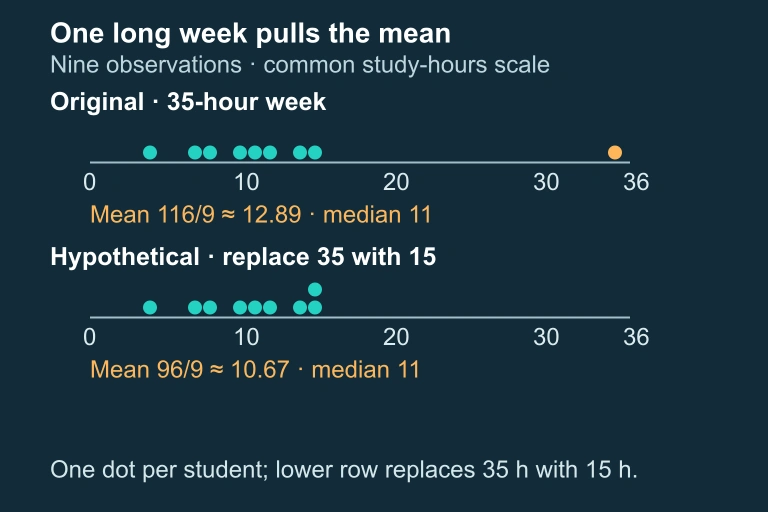One dot per student on two common-scale study-hour plots. The hypothetical lower row replaces 35 hours with 15; means are about 12.89 and 10.67 while both medians are 11. One dot represents one student. The lower row is a hypothetical replacement of 35 study hours by 15 hours.

SECTION 7

Comparing Mean/SD versus Median/IQR

On the AP exam, the choice between reporting the mean and standard deviation or the median and IQR must be justified by the distribution's shape and the presence of outliers. The table below highlights the key properties of each pair.

Property	Mean & SD	Median & IQR
Resistance to outliers	Not resistant — extreme values pull both x̄ and s	Resistant — based on ordered positions, not magnitudes
Best for which distributions?	Roughly symmetric, no strong outliers	Skewed distributions or those with outliers
Uses all data values?	Yes — every observation contributes to x̄ and s	No — depends on rank positions, not exact values
Algebraic properties	Deviations from x̄ sum to zero; used in inference formulas	No simple algebraic identity; primarily descriptive
Effect of adding a constant c	x̄ shifts by c; s unchanged	Median shifts by c; IQR unchanged
Effect of multiplying by k > 0	x̄ multiplied by k; s multiplied by k	Median multiplied by k; IQR multiplied by k

Comparison of the two main pairs of summary statistics

✦

KEY TAKEAWAY

Think of the mean as a GPS average of all your errand locations — if one errand is 200 miles away, the 'average location' shifts dramatically. The median, by contrast, is like choosing the middle stop on a ranked list of distances — the faraway outlier barely moves it. For AP free-response questions, always state which summary pair you chose and justify your choice by referencing the shape of the distribution or the presence of outliers.

SECTION 8

Connections to Inference and Advanced Topics

Summary statistics are not merely descriptive — they form the building blocks of statistical inference. The sample mean x̄ and sample standard deviation s reappear throughout the course as inputs to confidence intervals and hypothesis tests. Understanding how these statistics behave across repeated samples leads directly to the concept of sampling distributions and the Central Limit Theorem.

Descriptive Concept	Inferential Extension
Sample mean x̄	Point estimator for the population mean μ; appears in one-sample t-tests and t-intervals
Sample standard deviation s	Estimates σ; used to compute the standard error of x̄: SE = s / √n
Shape assessment (skewness, outliers)	Determines whether Normal-based procedures are appropriate or whether the sample size is large enough for CLT to apply
Transforming data (adding/multiplying)	Combining random variables: E(X + Y) = E(X) + E(Y); Var(aX + b) = a²Var(X)

From descriptive statistics to inferential reasoning

When you encounter later topics like z-scores (measuring how many standard deviations a value lies from the mean) or the empirical rule (approximately 68-95-99.7% of data within 1-2-3 standard deviations for Normal distributions), remember that they rest on the summary statistics you learn here. A firm grasp of center and spread — and when each measure is appropriate — will pay dividends throughout every unit of the AP Statistics curriculum.

SECTION 9

Practice Problems

Question 1: CONCEPTUAL

A distribution of household incomes in a small town is strongly right-skewed. Which of the following is true about the relationship between the mean and the median of this distribution?

A. The mean is less than the median because the skew pulls the mean toward lower values.
B. The mean equals the median because both measure the center of the distribution.
C. The mean is greater than the median because the long right tail pulls the mean toward higher values.
D. The mean is greater than the median because the median is always smaller than the mean for any distribution.
E. The relationship cannot be determined without knowing the exact data values.

Show answer (C)

C is correct. In a right-skewed distribution, a few very large values (high incomes) pull the mean toward the right tail, making it larger than the median. A is incorrect because right skew pulls the mean toward higher, not lower, values. B is incorrect because mean and median generally differ when a distribution is skewed. D gives the right relationship for this scenario but the reasoning is wrong — the median is not always smaller; in a left-skewed distribution the median exceeds the mean. E is incorrect because the direction of the mean-median relationship can be determined from the shape alone.

Question 2: BASIC CALCULATION

The five-number summary for a data set is: Min = 12, Q₁ = 18, Median = 25, Q₃ = 33, Max = 47. What is the interquartile range, and would an observation of 60 be classified as an outlier using the 1.5 × IQR rule?

A. IQR = 15; 60 is not an outlier because it is within 1.5 × IQR of the median.
B. IQR = 15; 60 is an outlier because 60 > Q₃ + 1.5 × IQR = 55.5.
C. IQR = 35; 60 is not an outlier because the range is only 35.
D. IQR = 15; 60 is not an outlier because 60 < Q₃ + 1.5 × IQR = 57.
E. IQR = 7; 60 is an outlier because it exceeds the maximum of 47.

Show answer (B)

B is correct. IQR = Q₃ − Q₁ = 33 − 18 = 15. The upper fence is Q₃ + 1.5 × IQR = 33 + 22.5 = 55.5. Since 60 > 55.5, the observation of 60 is classified as an outlier. A incorrectly computes the IQR correctly but applies the 1.5 × IQR rule relative to the median instead of Q₃. C confuses IQR with the range (47 − 12 = 35). D has the right IQR but miscalculates the upper fence as 57 instead of 55.5. E incorrectly computes IQR as 7 and confuses the outlier rule with simply exceeding the maximum.

Question 3: INTERMEDIATE

A data set of 20 test scores has a mean of 74 and a standard deviation of 8. Every score is then increased by 5 points (a curve). What are the new mean and new standard deviation?

A. New mean = 79; new standard deviation = 13
B. New mean = 79; new standard deviation = 8
C. New mean = 74; new standard deviation = 8
D. New mean = 74; new standard deviation = 13
E. New mean = 79; new standard deviation = 3

Show answer (B)

B is correct. Adding a constant c to every observation shifts the mean by c (74 + 5 = 79) but does not change the standard deviation because the spread of the data — the distances between values — remains identical. A incorrectly adds 5 to both the mean and the standard deviation. C fails to shift the mean. D changes neither correctly. E subtracts 5 from the standard deviation, which has no mathematical basis. The key principle is: adding a constant affects measures of center but not measures of spread.

Question 4: APPLIED

4 pts

A nutritionist collects the daily calorie intake (in kilocalories) for a sample of 10 adult participants over one day: 1,800 2,100 1,950 2,400 2,050 1,750 2,200 2,350 3,800 2,000 (a) Calculate the mean and median calorie intake. (b) Calculate the IQR and determine whether any observations are outliers using the 1.5 × IQR rule. (c) The nutritionist reports: 'The typical participant consumed approximately 2,240 calories.' Is this an appropriate description of a typical participant's intake? Justify your answer using the summary statistics you calculated.

Show answer

Rubric (4 points): Point 1 (Mean and Median): Ordered data: 1750, 1800, 1950, 2000, 2050, 2100, 2200, 2350, 2400, 3800. Mean = 22,400/10 = 2,240 kcal. Median = (2,050 + 2,100)/2 = 2,075 kcal. Point 2 (IQR Calculation): Q₁ = median of lower five = 1,950; Q₃ = median of upper five = 2,350. IQR = 2,350 − 1,950 = 400. Point 3 (Outlier Identification): Upper fence = Q₃ + 1.5 × IQR = 2,350 + 600 = 2,950. Lower fence = Q₁ − 1.5 × IQR = 1,950 − 600 = 1,350. Since 3,800 > 2,950, the value 3,800 is an outlier. No values fall below 1,350. Point 4 (Justification): The nutritionist's reported value of 2,240 is the mean, which is pulled upward by the outlier at 3,800 kcal. Because the distribution is right-skewed (the mean exceeds the median and there is a high outlier), the median of 2,075 kcal is a more appropriate measure of the typical participant's intake. The nutritionist's description is misleading because it overstates what a typical participant consumed.

Question 5: CRITICAL THINKING

4 pts

A teacher reports the following summary statistics for a class of 30 students' scores on a quiz (out of 50 points): x̄ = 38, s = 6, Median = 40, Q₁ = 35, Q₃ = 44, Min = 10, Max = 49. (a) Without seeing the raw data, what can you infer about the shape of the distribution from the relationship between the mean and median and from the five-number summary? Explain your reasoning. (b) One student scored 10. Is this student's score an outlier according to the 1.5 × IQR rule? Show your work. (c) If the student who scored 10 had instead scored 30, describe qualitatively what would happen to each of the following: the mean, the median, the standard deviation, and the IQR. Justify each claim.

Show answer

Rubric (4 points): Point 1 (Shape inference): The mean (38) is less than the median (40), suggesting the distribution is left-skewed. Additionally, the distance from Q₁ to the median (40 − 35 = 5) is less than the distance from Q₁ to the minimum (35 − 10 = 25), indicating a longer left tail. The distance from the median to Q₃ (44 − 40 = 4) is comparable to Q₁ to the median, and Q₃ to Max (49 − 44 = 5) is short, confirming the left skew. Point 2 (Outlier check): IQR = Q₃ − Q₁ = 44 − 35 = 9. Lower fence = Q₁ − 1.5 × IQR = 35 − 13.5 = 21.5. Since 10 < 21.5, the score of 10 is an outlier. The upper fence = 44 + 13.5 = 57.5; no scores exceed this (max is 49). Point 3 (Effect on mean and standard deviation): If the score of 10 is changed to 30, the sum increases by 20, so the new mean = (30 × 38 + 20)/30 = 1160/30 ≈ 38.67, an increase. The standard deviation would decrease because the most extreme low value has moved closer to the mean, reducing the sum of squared deviations. Point 4 (Effect on median and IQR): The median is unlikely to change (or would change very slightly) because replacing one value in the lower tail with another value still in the lower half does not move the middle observations. Similarly, Q₁ and Q₃ are determined by the positions of the 8th and 23rd ordered values; changing the minimum to 30 would shift it upward in rank but is unlikely to change Q₁ or Q₃ unless the 8th ordered value itself changes. Therefore the IQR would remain the same or change negligibly, illustrating the resistance of median and IQR to changes in extreme values.

SUMMARY

Summary

Summary statistics condense a quantitative distribution into a few interpretable numbers. Measures of center include the mean (the balance point, sensitive to outliers) and the median (the middle value, resistant to outliers). Measures of spread include the standard deviation (average distance from the mean, non-resistant) and the IQR (width of the middle 50%, resistant). The five-number summary (Min, Q₁, Median, Q₃, Max) underlies the box plot and, combined with the 1.5 × IQR rule, identifies potential outliers.

For roughly symmetric distributions without outliers, report the mean and standard deviation. For skewed distributions or those with outliers, report the median and IQR. Adding a constant shifts the center but leaves spread unchanged; multiplying by a positive constant scales both center and spread. These transformation rules extend directly into the study of random variables and inference later in the AP Statistics curriculum.