Sampling Distributions for Differences in Sample Means - AP Statistics

SECTION 1

Historical Context & Motivation

Much of modern statistics grew out of a deceptively simple question: when we observe a difference between two groups, how do we know it isn't just noise? Agricultural scientists measuring crop yields across different fertilizer treatments, medical researchers comparing drug outcomes to placebos, and psychologists contrasting reaction times under varying conditions all faced the same inferential challenge. Quantifying the sampling variability of the difference between two sample means became one of the central problems of 20th-century statistics, ultimately enabling the two-sample t-procedures that appear throughout applied science.

1908 • Student's t-distribution

William Sealy Gosset, publishing under the pseudonym "Student," derived the t-distribution while working at the Guinness brewery, providing the first rigorous small-sample framework for comparing means.

1922 • Fisher Formalizes Sampling Theory

Ronald Fisher established the foundations of sampling distributions, maximum likelihood estimation, and the analysis of variance, framing the difference in means as a ratio of signal to noise.

1935 • Design of Experiments Published

Fisher's landmark book made randomization and controlled comparison the gold standard, showing that sampling distributions of differences in means underpin valid experimental inference.

1947 • Welch's Approximate t-test

Bernard Welch proposed an adjustment for unequal variances, refining how statisticians model the sampling distribution of x̄₁ − x̄₂ when σ₁ ≠ σ₂—the version now standard on the AP Statistics exam.

The conceptual thread running through this history is that a single observed difference x̄₁ − x̄₂ means little on its own; we need to know how much that difference would vary across all possible pairs of random samples. That is precisely what the sampling distribution of the difference in sample means describes, and mastering it is the gateway to two-sample inference on the AP Statistics exam.

SECTION 2

Core Principles & Definitions

Before diving into formulas, it is essential to internalize the building blocks. If you already understand the sampling distribution of a single sample mean, extending to the difference of two means requires just a few additional ideas—each grounded in the properties of independent random variables.

Sampling Distribution of x̄₁ − x̄₂

The probability distribution of all possible values of the difference in sample means when two independent random samples of sizes n₁ and n₂ are drawn from their respective populations.

Center: μ₁ − μ₂

The mean of the sampling distribution equals the difference of the population means, ensuring the statistic is an unbiased estimator of the parameter of interest.

Spread: Standard Error

When samples are independent, variances add: SE = √(σ₁²/n₁ + σ₂²/n₂). Larger samples reduce this standard error and tighten the distribution.

Shape: Approximately Normal

By the Central Limit Theorem, the shape approaches a normal distribution when both n₁ and n₂ are sufficiently large—or when both parent populations are themselves normal.

Independence Condition

The two samples must be independent of each other, and observations within each sample must be independent. For sampling without replacement, the 10% condition (n < 0.10N) must hold for each population.

✦

KEY TAKEAWAY

Think of the difference x̄₁ − x̄₂ like the net score in a two-round competition. Each round has its own variability—some days your team scores high, some days low—but the variability of the difference between rounds combines both sources of uncertainty. In statistics, when two independent quantities each wobble, the wobble in their difference is the square root of the sum of their individual squared wobbles. That is why variances add—even when we subtract means.

SECTION 3

Visual Explanation

The diagram below illustrates how two separate population distributions give rise to their own sampling distributions of x̄, and how combining those two sampling distributions produces the sampling distribution of x̄₁ − x̄₂. Notice that the center of the bottom distribution sits at μ₁ − μ₂, and its spread reflects the combined uncertainty from both samples.

Two independent populations (cyan and pink) each contribute sampling variability. When we take the difference of sample means, the resulting sampling distribution (violet) is centered at μ₁ − μ₂ with a standard error that combines both sources of variability via the addition of variances.

Several features of this diagram deserve emphasis. First, the violet curve at the bottom is narrower relative to the original populations because sampling distributions are always less variable than the parent distributions from which they arise—the factor of 1/n inside each variance term ensures this. Second, the shape is approximately normal even if the two parent populations are not perfectly normal, provided both sample sizes are large enough (typically n₁ ≥ 30 and n₂ ≥ 30 serves as a working guideline, though smaller samples suffice when the populations are unimodal and roughly symmetric). Third, the center of μ₁ − μ₂ = 10 is deterministic: no matter how many times we repeat the sampling process, the average of all possible differences in sample means equals the true difference in population means.

SECTION 4

Mathematical Framework

The properties of the sampling distribution of x̄₁ − x̄₂ follow directly from two foundational results: the linearity of expectation and the variance addition rule for independent random variables. Let X̄₁ and X̄₂ be the sample means from two independent random samples of sizes n₁ and n₂ drawn from populations with means μ₁, μ₂ and standard deviations σ₁, σ₂ respectively.

MEAN OF THE DIFFERENCE

μ_{x̄₁ − x̄₂} = μ₁ − μ₂

The expected value of the difference in sample means equals the difference in population means. This follows from E(X̄₁ − X̄₂) = E(X̄₁) − E(X̄₂) = μ₁ − μ₂ by linearity of expectation.

STANDARD ERROR (POPULATION σ KNOWN)

σ_{x̄₁ − x̄₂} = √(σ₁²/n₁ + σ₂²/n₂)

Because X̄₁ and X̄₂ are independent, Var(X̄₁ − X̄₂) = Var(X̄₁) + Var(X̄₂) = σ₁²/n₁ + σ₂²/n₂. The standard error is the square root of this sum. Note that variances add even though we are subtracting means—this is a critical conceptual point.

STANDARD ERROR (σ ESTIMATED FROM SAMPLES)

SE_{x̄₁ − x̄₂} = √(s₁²/n₁ + s₂²/n₂)

In practice, population standard deviations are unknown. We replace σ₁ and σ₂ with the sample standard deviations s₁ and s₂. This estimated standard error is used in t-procedures for two-sample inference.

SHAPE CONDITION (CLT)

(x̄₁ − x̄₂) ~ Approx. Normal when n₁ ≥ 30 and n₂ ≥ 30 (or both populations normal)

The Central Limit Theorem guarantees approximate normality for large samples regardless of population shape. When the parent populations are themselves normal, the sampling distribution of x̄₁ − x̄₂ is exactly normal for any sample sizes.

⚠

Why Variances Add for Differences

Students often ask: "If we subtract the means, shouldn't we subtract the variances?" The answer is no. Variance measures squared spread, and subtracting one variable from another does not reduce uncertainty—it compounds it. If you wobble left and your friend wobbles right, the distance between you wobbles more, not less. Formally, Var(A − B) = Var(A) + Var(B) − 2Cov(A, B), and when A and B are independent the covariance term is zero, leaving Var(A) + Var(B).

SECTION 5

Conditions & Checking Assumptions

On the AP Statistics exam, you will be expected to verify three categories of conditions before using the normal model for x̄₁ − x̄₂. Free-response rubrics consistently award points for explicitly stating and checking these conditions. The following diagram and table break them down clearly.

The three-condition checklist — Random, Independent, Normal — must all be verified before applying the normal model to x̄₁ − x̄₂. This flowchart mirrors the structure expected in AP free-response answers.

Condition	What to Check	What to Write on the Exam
Random	Both samples come from random selection or random assignment in an experiment.	"We are told that both samples were selected via SRS from their respective populations."
Independent (10%)	The two samples are independent of each other, and each n is less than 10% of its population N.	"It is reasonable that n₁ = 40 < 10% of all [population 1] and n₂ = 50 < 10% of all [population 2], so independence holds."
Normal (Large Counts / CLT)	n₁ ≥ 30 and n₂ ≥ 30, or the parent populations are approximately normal with no strong skew/outliers.	"Since n₁ = 40 ≥ 30 and n₂ = 50 ≥ 30, the CLT ensures the sampling distribution of x̄₁ − x̄₂ is approximately normal."

Conditions checklist with AP-exam-style phrasing

Participants wear headphones at matching task stations while a researcher distributes cards. Measurements taken from the same person remain linked. Compare within-person differences instead of treating the two columns as independent samples.

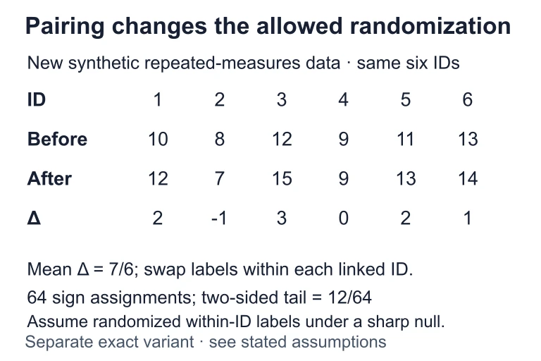Six linked before-and-after pairs become six differences; within-ID sign swaps generate 64 assignments with 12 in the marked absolute tail. Suppose the same six IDs have differences 2, −1, 3, 0, 2 and 1, averaging 7/6. Under a sharp zero-effect null with randomized or exchangeable within-ID labels, 2⁶ = 64 sign assignments are allowed; 12 have absolute mean at least 7/6. Repeated measurement alone does not establish that exchangeability.

SECTION 6

Worked Example

A researcher wants to compare the average time (in minutes) that college students spend studying per day at two universities. A random sample of 36 students from University A yields x̄₁ = 142 minutes with s₁ = 28 minutes. An independent random sample of 45 students from University B yields x̄₂ = 128 minutes with s₂ = 32 minutes. Describe the sampling distribution of x̄₁ − x̄₂ and find the probability that the difference in sample means exceeds 25 minutes, assuming the true difference in population means is μ₁ − μ₂ = 14.

Describing and Using the Sampling Distribution of x̄₁ − x̄₂

1
Step 1 — Verify Conditions

Random: Both samples are described as random samples. Independent: The samples come from separate universities and are independent. Since 36 < 10% of all students at University A and 45 < 10% of all students at University B (assuming each has more than 360 and 450 students, respectively), the 10% condition is satisfied for both. Normal: n₁ = 36 ≥ 30 and n₂ = 45 ≥ 30, so the CLT ensures approximate normality.
2
Step 2 — State the Center (Mean)

The mean of the sampling distribution of x̄₁ − x̄₂ is μ₁ − μ₂ = 14 minutes.

μ_{x̄₁ − x̄₂} = 14 minutes
3
Step 3 — Compute the Standard Error

Using the sample standard deviations as estimates for σ₁ and σ₂: SE = √(s₁²/n₁ + s₂²/n₂) = √(28²/36 + 32²/45) = √(784/36 + 1024/45) = √(21.778 + 22.756) = √44.534 ≈ 6.673 minutes.

SE ≈ 6.673 minutes
4
Step 4 — State the Sampling Distribution

The sampling distribution of x̄₁ − x̄₂ is approximately Normal(14, 6.673). In notation: x̄₁ − x̄₂ ~ N(14, 6.673).
5
Step 5 — Compute the z-score and Probability

We want P(x̄₁ − x̄₂ > 25). The z-score is z = (25 − 14) / 6.673 = 11 / 6.673 ≈ 1.649. Using the standard normal table or calculator: P(Z > 1.649) ≈ 0.0497.

P(x̄₁ − x̄₂ > 25) ≈ 0.0497
6
Step 6 — Interpret in Context

If the true difference in mean study times between the two universities is 14 minutes, there is approximately a 5.0% probability of observing a difference in sample means exceeding 25 minutes from samples of these sizes.

SECTION 7

Common Errors & Exam Pitfalls

AP Statistics scorers report that certain mistakes recur year after year on free-response questions involving two-sample inference. Understanding these pitfalls in advance can prevent lost points and deepen your conceptual grasp of sampling distributions.

Common Error	Why It's Wrong	Correct Approach
Subtracting standard errors	Writing SE = √(σ₁²/n₁) − √(σ₂²/n₂) confuses standard deviations with variances. Subtraction of SDs is not a valid operation for combining independent variabilities.	Add the variances first, then take the square root: SE = √(σ₁²/n₁ + σ₂²/n₂).
Subtracting variances	Writing Var = σ₁²/n₁ − σ₂²/n₂ because the statistic involves subtraction. Variances always add for independent random variables, regardless of whether we add or subtract the variables.	Var(X̄₁ − X̄₂) = Var(X̄₁) + Var(X̄₂) = σ₁²/n₁ + σ₂²/n₂.
Forgetting to check conditions	Jumping straight to calculation without verifying Random, Independent, and Normal conditions. This typically costs 1–2 rubric points on FRQs.	Always state all three conditions and show evidence for each before proceeding with calculations.
Confusing σ and s	Using population parameters σ₁ and σ₂ in formulas when only sample statistics s₁ and s₂ are available, or vice versa.	Use σ only when population standard deviations are explicitly given; otherwise use s and note that the result is an estimated standard error.
Context-free interpretation	Stating a probability without referring to what x̄₁ − x̄₂ represents in the problem context.	Always interpret probabilities in context: "There is a 5% chance the difference in sample mean study times exceeds 25 minutes, assuming…"

Common exam errors and corrections for two-sample mean inference

📝

EXAM STRATEGY

Think of the AP scoring rubric as a recipe: the conditions check is one ingredient, the formula is another, the computation is a third, and the contextual interpretation is the final ingredient. Omitting any one of them produces an incomplete dish and costs points. The most reliable exam habit is to always write: Conditions → Formula → Calculation → Interpretation in that order.

SECTION 8

Connection to Two-Sample t-Inference

Everything developed in this lesson about the sampling distribution of x̄₁ − x̄₂ is the theoretical foundation upon which two-sample t-confidence intervals and two-sample t-tests are built. When you construct a confidence interval for μ₁ − μ₂ or conduct a hypothesis test about whether μ₁ − μ₂ equals zero, you are using the sampling distribution to quantify how far the observed x̄₁ − x̄₂ might plausibly fall from the true parameter.

Concept	This Lesson (Sampling Distribution)	Next Topic (Two-Sample t-Procedures)
Parameter of interest	μ₁ − μ₂ (difference in population means)	Same: μ₁ − μ₂
Statistic	x̄₁ − x̄₂	Same: x̄₁ − x̄₂
Standard error	σ known: √(σ₁²/n₁ + σ₂²/n₂); σ unknown: √(s₁²/n₁ + s₂²/n₂)	Always estimated: √(s₁²/n₁ + s₂²/n₂)
Distribution used	Normal (z) when σ known; t when σ estimated	t-distribution with Welch's df: df ≈ (s₁²/n₁ + s₂²/n₂)² / [(s₁²/n₁)²/(n₁−1) + (s₂²/n₂)²/(n₂−1)]
Primary use	Describing the distribution and computing probabilities about x̄₁ − x̄₂	Constructing confidence intervals and performing hypothesis tests for μ₁ − μ₂

Bridge from sampling distributions to formal two-sample inference

The key transition is straightforward: once you know how to describe the center, spread, and shape of the sampling distribution of x̄₁ − x̄₂, constructing a confidence interval simply means placing a margin of error around the observed difference, and conducting a hypothesis test means measuring how many standard errors the observed difference lies from the hypothesized value (usually zero). The Welch's degrees of freedom formula adjusts for the fact that when we estimate σ from data, the normal model slightly understates the tails; the t-distribution corrects this. On the AP exam, your calculator handles the df computation, but understanding the sampling distribution from this lesson is what makes the entire procedure meaningful.

SECTION 9

Practice Problems

Question 1: CONCEPTUAL

Two independent random samples are taken from populations with means μ₁ and μ₂ and standard deviations σ₁ and σ₂. Which of the following correctly describes the standard deviation of the sampling distribution of x̄₁ − x̄₂?

A. σ₁/√n₁ − σ₂/√n₂
B. √(σ₁²/n₁ − σ₂²/n₂)
C. √(σ₁²/n₁ + σ₂²/n₂)
D. (σ₁ + σ₂)/√(n₁ + n₂)
E. √(σ₁² + σ₂²)/√(n₁ + n₂)

Show answer (C)

C is correct. For independent random variables, Var(X̄₁ − X̄₂) = Var(X̄₁) + Var(X̄₂) = σ₁²/n₁ + σ₂²/n₂, so the standard deviation is √(σ₁²/n₁ + σ₂²/n₂). A is wrong because you cannot subtract standard deviations—standard deviations do not combine linearly. B is wrong because variances add, not subtract, even when we compute a difference in means. D incorrectly pools standard deviations and sample sizes. E incorrectly sums variances across populations before dividing by the combined sample size, which is not how independent sampling works.

Question 2: BASIC CALCULATION

A sample of n₁ = 49 observations from Population 1 has x̄₁ = 85 and σ₁ = 14. An independent sample of n₂ = 64 from Population 2 has x̄₂ = 78 and σ₂ = 16. What is the standard error of x̄₁ − x̄₂?

A. 2.00
B. 2.83
C. 4.00
D. 8.00
E. 30.00

Show answer (B)

B is correct. SE = √(σ₁²/n₁ + σ₂²/n₂) = √(14²/49 + 16²/64) = √(196/49 + 256/64) = √(4 + 4) = √8 ≈ 2.83. A (2.00) results from only using one of the two variance terms. C (4.00) is the sum of the two individual standard errors rather than the square root of the sum of variances. D (8.00) represents the variance (the sum before taking the square root). E (30.00) appears to add the standard deviations directly (14 + 16), which is not valid.

Question 3: INTERMEDIATE

The mean blood pressure for a random sample of 40 runners is x̄₁ = 118 mmHg (s₁ = 10), and for a random sample of 35 non-runners is x̄₂ = 126 mmHg (s₂ = 12). Assuming the true difference is μ₁ − μ₂ = −8, what is the approximate probability that the observed difference x̄₁ − x̄₂ will be more extreme than −15 mmHg (i.e., P(x̄₁ − x̄₂ < −15))?

A. 0.0082
B. 0.0033
C. 0.0052
D. 0.0250
E. 0.0500

Show answer (B)

B is correct. The true difference is μ₁ − μ₂ = −8, and we need to find P(x̄₁ − x̄₂ < −15). First, compute the standard error of the difference: SE = √(s₁²/n₁ + s₂²/n₂) = √(10²/40 + 12²/35) = √(100/40 + 144/35) = √(2.5 + 4.1143) = √6.6143 ≈ 2.572. Next, compute the z-score: z = (−15 − (−8))/2.572 = −7/2.572 ≈ −2.72. Using the standard normal table, P(Z < −2.72) ≈ 0.0033. A (0.0082) corresponds to approximately z ≈ −2.40, which would result from an inflated SE, such as mistakenly using larger standard deviations or smaller sample sizes. C (0.0052) corresponds to approximately z ≈ −2.56, which could arise from a minor arithmetic error in computing the SE. D (0.0250) corresponds to approximately z ≈ −1.96, which would result from a substantially larger SE or a different value substituted for the difference. E (0.0500) corresponds to z ≈ −1.645, which drastically underestimates how far −15 is from −8 relative to the SE.

Question 4: APPLIED

7 pts

A pharmaceutical company is testing a new pain medication. In a randomized experiment, 50 patients receiving the new drug report a mean pain reduction of x̄₁ = 4.8 points (s₁ = 2.1) on a 10-point scale, while 55 patients receiving a placebo report a mean pain reduction of x̄₂ = 3.1 points (s₂ = 2.5). (a) Verify all conditions required to describe the sampling distribution of x̄₁ − x̄₂. (b) Describe the sampling distribution of x̄₁ − x̄₂ (center, spread, and shape). Use the observed sample statistics as estimates where necessary. (c) The company considers the drug "meaningfully better" if the true mean difference exceeds 1.0 point. Using the sampling distribution described in part (b), find the probability that x̄₁ − x̄₂ would be less than 1.0 if the true difference were μ₁ − μ₂ = 1.7. (d) Interpret your answer from part (c) in the context of the study.

Show answer

Rubric (7 points): Part (a) — Conditions (2 points): • (1 pt) Random: Patients were randomly assigned to treatment groups in a randomized experiment, satisfying the randomization condition. • (½ pt) Independent: The two groups are independent because of random assignment. Since sampling is from a treatment context (not from a finite population), the 10% condition is automatically satisfied. • (½ pt) Normal: n₁ = 50 ≥ 30 and n₂ = 55 ≥ 30, so the CLT guarantees approximate normality of the sampling distribution. Part (b) — Describe the sampling distribution (2 points): • (½ pt) Center: μ_{x̄₁ − x̄₂} = μ₁ − μ₂ (the true difference in population means). • (1 pt) Spread: SE = √(s₁²/n₁ + s₂²/n₂) = √(2.1²/50 + 2.5²/55) = √(4.41/50 + 6.25/55) = √(0.0882 + 0.1136) = √0.2018 ≈ 0.449. • (½ pt) Shape: Approximately normal, justified by CLT with both samples ≥ 30. So x̄₁ − x̄₂ ~ Approx. Normal(μ₁ − μ₂, 0.449). Part (c) — Probability calculation (2 points): • (1 pt) z = (1.0 − 1.7)/0.449 = −0.7/0.449 ≈ −1.559. • (1 pt) P(x̄₁ − x̄₂ < 1.0) = P(Z < −1.559) ≈ 0.0596. Part (d) — Interpretation in context (1 point): • (1 pt) If the true mean difference in pain reduction between the drug and placebo groups is 1.7 points, there is approximately a 6.0% probability that the observed difference in sample mean pain reductions would be less than 1.0 point with samples of these sizes. This suggests that if the drug truly provides a 1.7-point advantage, it is unlikely (but possible) that the study would fail to observe at least a 1.0-point difference.

Question 5: CRITICAL THINKING

7 pts

A researcher plans to compare the mean commute times (in minutes) of employees in City A versus City B. She wants the standard error of x̄₁ − x̄₂ to be no greater than 2.0 minutes. From pilot studies, she estimates σ₁ ≈ 12 minutes and σ₂ ≈ 15 minutes. She plans to use equal sample sizes (n₁ = n₂ = n). (a) Derive an expression for n in terms of σ₁, σ₂, and the desired SE. (b) Calculate the minimum n (per group) required to achieve SE ≤ 2.0 minutes. (c) Suppose budget constraints limit her to n = 50 per group. What would the standard error be? Explain whether this SE is adequate if she needs to detect a true difference of μ₁ − μ₂ = 5 minutes with reasonable confidence. (d) A colleague suggests that instead of equal sample sizes, she should allocate more observations to the population with larger variability. Justify or refute this claim using the SE formula.

Show answer

Rubric (7 points): Part (a) — Derivation (2 points): • (1 pt) Start with SE = √(σ₁²/n + σ₂²/n) = √((σ₁² + σ₂²)/n). • (1 pt) Set √((σ₁² + σ₂²)/n) ≤ SE_max. Square both sides: (σ₁² + σ₂²)/n ≤ SE_max². Solve for n: n ≥ (σ₁² + σ₂²)/SE_max². Part (b) — Calculation (1 point): • (1 pt) n ≥ (12² + 15²)/2² = (144 + 225)/4 = 369/4 = 92.25. Since n must be a whole number, n ≥ 93 per group (round up). Part (c) — Evaluate n = 50 (2 points): • (1 pt) SE = √((144 + 225)/50) = √(369/50) = √7.38 ≈ 2.717 minutes. • (1 pt) With SE ≈ 2.72 and a true difference of 5 minutes, the z-score for testing H₀: μ₁ − μ₂ = 0 would be approximately 5/2.72 ≈ 1.84, which places the observed difference only about 1.84 standard errors from zero. This would yield a one-sided p-value around 0.033 — marginally significant at α = 0.05 but potentially underpowered for a two-sided test (p ≈ 0.066). The researcher should consider whether this level of precision is adequate for her inferential goals. Part (d) — Optimal allocation (2 points): • (1 pt) The claim is correct. The SE formula is √(σ₁²/n₁ + σ₂²/n₂). Since σ₂ > σ₁, the term σ₂²/n₂ contributes more to the total SE. Increasing n₂ reduces this larger term more efficiently than increasing n₁ by the same amount. • (1 pt) Formally, for a fixed total sample size N = n₁ + n₂, the SE is minimized when n₁/n₂ = σ₁/σ₂ (Neyman allocation). Here, that ratio would be 12/15 = 0.8, meaning roughly 44% of observations should go to City A and 56% to City B, allocating more to the more variable population as the colleague suggests.

SUMMARY

Lesson Summary

Summary

The sampling distribution of x̄₁ − x̄₂ describes how the difference in sample means varies across all possible pairs of independent random samples. Its center is μ₁ − μ₂, making it an unbiased estimator of the true difference in population means. Its standard error is √(σ₁²/n₁ + σ₂²/n₂) — critically, variances always add for independent random variables, even when means are subtracted. Its shape is approximately normal when both sample sizes are at least 30 (by the Central Limit Theorem) or when both populations are normal.

Before applying this model, always verify the three conditions: Random (both samples arise from random selection or random assignment), Independent (the two samples are independent and each satisfies the 10% condition), and Normal (the CLT applies or populations are normal). This sampling distribution is the theoretical backbone of two-sample t-intervals and t-tests, which you will encounter next in the AP Statistics curriculum.