Sampling Distributions for Sample Proportions - AP Statistics

SECTION 1

Historical Context & Motivation

The question of how reliably a sample reflects a larger population has occupied mathematicians and scientists for centuries. When a pollster surveys 1,000 voters and reports that 54% support a candidate, the natural follow-up is: how close is that 54% to the true proportion in the entire electorate? Answering this question requires understanding the sampling distribution of the sample proportion—the probability distribution that describes how p̂ (the sample proportion) behaves across all possible random samples of a given size. The development of this idea spans several centuries and reflects a deep interplay between probability theory, mathematical analysis, and practical statistical reasoning.

1713 • Bernoulli's Ars Conjectandi

Jakob Bernoulli published a posthumous proof of the Law of Large Numbers, establishing that as sample size grows, the sample proportion converges to the true population proportion. This was the first rigorous connection between samples and populations.

1733 • De Moivre's Normal Approximation

Abraham de Moivre showed that the binomial distribution could be approximated by a bell-shaped curve for large n, laying the mathematical groundwork for using the normal distribution to model sample proportions.

1812 • Laplace Generalizes the CLT

Pierre-Simon Laplace extended de Moivre's result into the Central Limit Theorem, demonstrating that sums and averages of independent random variables tend toward normality regardless of the original distribution—making the normal model broadly applicable.

1935 • Neyman's Confidence Intervals

Jerzy Neyman formalized confidence interval theory, directly leveraging the sampling distribution of p̂ to provide rigorous interval estimates for population proportions—a technique central to modern survey methodology.

These historical developments converge on a single powerful idea: even though individual samples are imperfect reflections of their populations, the pattern of variation across many samples is predictable. This predictability is precisely what allows us to quantify uncertainty through margins of error, confidence intervals, and hypothesis tests. The central question this lesson addresses is: if we know the true population proportion p, what can we say about the shape, center, and spread of p̂ across all possible samples of size n?

SECTION 2

Core Principles & Definitions

Before examining the mathematical machinery, it is essential to establish the foundational concepts that govern how sample proportions behave. Each principle below builds upon the preceding one: we start with the distinction between a parameter and a statistic, move to the concept of a sampling distribution, and then state the conditions under which a remarkably clean normal model applies.

Parameter vs. Statistic

The population proportion p is a fixed parameter describing the true fraction of successes in the population. The sample proportion p̂ (read 'p-hat') is a statistic computed from data: p̂ = X/n, where X is the count of successes in n independent trials. Because p̂ changes from sample to sample, it is a random variable.

Sampling Distribution Defined

The sampling distribution of p̂ is the probability distribution of p̂ over every possible random sample of size n drawn from the population. It tells us which values of p̂ are likely, which are rare, and how tightly p̂ clusters around the true p.

Center: Unbiasedness

The mean of the sampling distribution equals the population proportion: μ_p̂ = p. This means p̂ is an unbiased estimator of p: on average, across many samples, p̂ hits the target exactly.

Spread: Standard Deviation

The standard deviation of p̂ is σ_p̂ = √(p(1 − p)/n). Larger samples produce smaller spread, meaning p̂ concentrates more tightly around p.

Shape: Normal Approximation

When the Large Counts Condition is met (np ≥ 10 and n(1 − p) ≥ 10), the sampling distribution of p̂ is approximately normal. This condition ensures enough expected successes and failures for the bell curve to apply.

✦

KEY TAKEAWAY

Think of taking repeated samples like repeatedly launching darts at a target. The center of the dartboard is p, and each throw lands at some p̂. An unbiased estimator means the darts are centered on the bullseye—no systematic pull in any direction. The standard deviation σ_p̂ describes how tightly the darts cluster: larger n is like a more skilled thrower whose darts group tightly around the center. The normal model describes the circular, bell-shaped cloud formed by thousands of throws.

SECTION 3

Visual Explanation: From Population to Sampling Distribution

The following diagram illustrates the conceptual process of constructing a sampling distribution. Imagine a large population with true proportion p = 0.40. We repeatedly draw random samples of size n = 50, compute p̂ for each sample, and then plot the distribution of all those p̂ values. The resulting histogram forms the sampling distribution, which—when the Large Counts Condition is satisfied—takes on the characteristic bell shape of a normal distribution centered at p.

The diagram traces the process from a population with p = 0.40, through repeated sampling at n = 50, to the resulting bell-shaped sampling distribution of p̂. The dashed pink line marks the center at p = 0.40, while the amber dashed lines indicate ±1 standard deviation (σ_p̂ ≈ 0.069).

Notice several important features in the diagram. First, each individual sample produces a different p̂ value—0.38, 0.44, 0.36, and so on—reflecting natural sampling variability. Second, when we aggregate thousands of these p̂ values, the histogram forms a smooth, symmetric bell curve centered on the true population proportion p = 0.40. Third, the spread of this distribution—governed by σ_p̂ = √(0.40 × 0.60 / 50) ≈ 0.069—quantifies how much p̂ typically deviates from p in a single sample. About 68% of all sample proportions fall within one standard deviation of the center, and about 95% fall within two standard deviations.

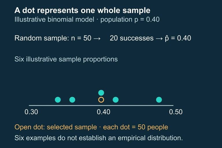Six illustrative sample proportions 0.34,0.36,0.40,0.40,0.42,0.48, with one dot per whole sample. The selected example has 20 successes out of 50. Each plotted sampling-distribution mark summarizes a whole 50-person sample rather than one student; the displayed small sequence is illustrative. The wider sampling distribution has standard error about 0.069.

SECTION 4

Mathematical Framework

The sampling distribution of p̂ arises from the binomial distribution. If each observation in a sample of size n independently has probability p of being a "success," then the count X of successes follows a Binomial(n, p) distribution. Since p̂ = X/n, the properties of p̂ follow directly from those of X. The three key formulas below describe the center, spread, and approximate shape of the distribution of p̂.

MEAN OF THE SAMPLING DISTRIBUTION

μ_p̂ = p

The expected value of p̂ equals the population proportion p, confirming that p̂ is an unbiased estimator. No matter the sample size, the center of the sampling distribution always aligns with the true parameter.

STANDARD DEVIATION OF THE SAMPLING DISTRIBUTION

σ_p̂ = √( p(1 − p) / n )

Here p is the population proportion and n is the sample size. This formula assumes either an infinite population or sampling with replacement. When sampling without replacement from a finite population of size N, multiply by the finite population correction factor √((N − n)/(N − 1)). The correction is negligible when n < 10% of N (the 10% Condition).

NORMAL APPROXIMATION (LARGE COUNTS CONDITION)

p̂ ~ approximately N( p, √(p(1−p)/n) ) when np ≥ 10 and n(1−p) ≥ 10

The Large Counts Condition ensures that the expected number of successes (np) and expected number of failures (n(1 − p)) are both at least 10. When this holds, the binomial-based distribution of p̂ is well-approximated by the normal distribution, enabling us to use z-scores for probability calculations.

Z-SCORE FOR A SAMPLE PROPORTION

z = (p̂ − p) / √( p(1 − p) / n )

This standardization converts a p̂ value into a z-score, measuring how many standard deviations p̂ lies from the center p. This z-score is essential for computing probabilities and performing hypothesis tests about population proportions.

⚠

Conditions Checklist for AP Exams

On the AP Statistics exam, you must verify three conditions before applying the normal model for p̂: (1) Random — the data come from a random sample or randomized experiment; (2) Independence (10% Condition) — when sampling without replacement, n < 10% of the population; (3) Large Counts — np ≥ 10 and n(1 − p) ≥ 10. Failing to state and verify these conditions is one of the most common point deductions on free-response questions.

SECTION 5

How Sample Size and Population Proportion Affect the Distribution

The shape and spread of the sampling distribution of p̂ depend on two quantities: the sample size n and the population proportion p. Understanding their effects is critical both for designing studies and for reasoning about results on the AP exam. The diagram below shows how the sampling distribution changes as n increases, holding p constant at 0.30.

Three normal curves for p = 0.30 at sample sizes n = 25 (red, σ ≈ 0.092), n = 100 (amber, σ ≈ 0.046), and n = 400 (cyan, σ ≈ 0.023). As n increases, the distribution narrows dramatically—quadrupling n halves the standard deviation.

The visual makes a crucial relationship concrete: since σ_p̂ = √(p(1 − p)/n), the standard deviation is inversely proportional to the square root of n. This means quadrupling the sample size cuts the standard deviation in half. Going from n = 25 to n = 100 (a factor of 4) reduces σ_p̂ from 0.092 to 0.046—exactly half. This square-root relationship has practical implications for survey design: achieving twice the precision requires four times the sample size, which means four times the cost.

Sample Size (n)	σ_p̂ (when p = 0.30)	Large Counts Met?	Approx. 95% Range for p̂
10	0.145	No (np = 3)	Normal model not appropriate
50	0.065	Yes (np = 15, n(1−p) = 35)	(0.17, 0.43)
200	0.032	Yes (np = 60, n(1−p) = 140)	(0.24, 0.36)
1000	0.014	Yes (np = 300, n(1−p) = 700)	(0.27, 0.33)

Sampling distribution characteristics for p = 0.30 at various sample sizes

The value of p also affects the standard deviation and the validity of the normal approximation. The product p(1 − p) is maximized when p = 0.50 and decreases symmetrically as p approaches 0 or 1. When p is extreme (near 0 or 1), the sampling distribution is more skewed and requires a larger n to satisfy the Large Counts Condition. For instance, with p = 0.05, you would need n ≥ 200 to reach np = 10, whereas with p = 0.50, even n = 20 suffices.

SECTION 6

Worked Example: Finding a Probability for p̂

A large university reports that 65% of its students graduate in four years. A researcher takes a simple random sample of 150 students. What is the probability that the sample proportion of four-year graduates exceeds 0.70?

Computing P(p̂ > 0.70) Using the Normal Model

1
Step 1 — Identify Given Values

Population proportion: p = 0.65. Sample size: n = 150. We want P(p̂ > 0.70).

p = 0.65, n = 150, target p̂ = 0.70
2
Step 2 — Verify Conditions

Random: The problem states the sample is a simple random sample. ✓ Independence (10% Condition): A large university has far more than 1,500 students, so 150 < 10% of the population. ✓ Large Counts: np = 150 × 0.65 = 97.5 ≥ 10 ✓ and n(1 − p) = 150 × 0.35 = 52.5 ≥ 10 ✓. All conditions are satisfied.

All three conditions met — normal model is appropriate
3
Step 3 — Compute Mean and Standard Deviation

Mean: μ_p̂ = p = 0.65. Standard deviation: σ_p̂ = √(0.65 × 0.35 / 150) = √(0.2275 / 150) = √(0.001517) ≈ 0.03894.

μ_p̂ = 0.65, σ_p̂ ≈ 0.0389
4
Step 4 — Compute the z-Score

z = (p̂ − p) / σ_p̂ = (0.70 − 0.65) / 0.03894 = 0.05 / 0.03894 ≈ 1.284.

z ≈ 1.28
5
Step 5 — Find the Probability

Using the standard normal table or calculator: P(Z > 1.28) = 1 − P(Z ≤ 1.28) = 1 − 0.8997 ≈ 0.1003. On a TI-84, you could compute normalcdf(0.70, 1E99, 0.65, 0.03894) ≈ 0.0994.

P(p̂ > 0.70) ≈ 0.10, or about 10%
6
Step 6 — Interpret in Context

If the true four-year graduation rate is 65%, there is approximately a 10% chance that a random sample of 150 students would yield a sample proportion of four-year graduates exceeding 0.70. This result is somewhat unusual but not extraordinarily rare—it would happen about 1 in 10 times by chance alone.

SECTION 7

Common Errors & Misconceptions

Even students with a solid grasp of the formulas frequently lose points on the AP exam due to subtle but important errors. The table below catalogues the most common mistakes and their corrections, drawing on patterns observed in released AP scoring guidelines.

Common Error	Why It's Wrong	Correct Approach
Using p̂ (from sample data) in the standard deviation formula when p is known	The standard deviation σ_p̂ requires the true population proportion p. Substituting p̂ yields the standard error, which is appropriate for confidence intervals but not when the population parameter is known (e.g., hypothesis testing).	Use σ_p̂ = √(p(1−p)/n) when p is given. Use SE = √(p̂(1−p̂)/n) only when estimating from data.
Confusing the distribution of X with the distribution of p̂	X ~ Binomial(n, p) counts successes; p̂ = X/n is a proportion. Their means and standard deviations differ by a factor of n.	For p̂: mean = p, SD = √(p(1−p)/n). For X: mean = np, SD = √(np(1−p)). Be clear about which you are modeling.
Forgetting to check or state the conditions	Applying the normal model without verifying the Random, 10%, and Large Counts conditions loses points on FRQs. The rubric typically dedicates 1–2 points to conditions alone.	Always state all three conditions with context-specific verification: name the condition, show the numerical check, and state whether it is satisfied.
Claiming the sampling distribution is always normal	When np or n(1−p) is less than 10, the distribution of p̂ is noticeably skewed and the normal model provides poor approximations, especially in the tails.	State that the distribution is approximately normal only when the Large Counts Condition is met. For small samples or extreme p, use the exact binomial distribution.
Believing larger samples change the population distribution	Increasing n does not alter the population. It makes the sampling distribution of the statistic narrower and more normal, but the underlying population remains unchanged.	Distinguish clearly between the population distribution (fixed) and the sampling distribution of p̂ (depends on n). Larger n → narrower sampling distribution, not a different population.

Common errors and misconceptions about the sampling distribution of p̂

✦

KEY TAKEAWAY

Think of the difference between σ_p̂ and SE like the distinction in engineering between a theoretical blueprint and an as-built measurement. The standard deviation σ_p̂ is the blueprint—it uses the known parameter p to describe ideal behavior. The standard error SE is the as-built version—it plugs in p̂ because p is unknown. On the AP exam, use σ_p̂ for hypothesis tests (where p is specified by H₀) and SE for confidence intervals (where p must be estimated from the sample).

SECTION 8

Connection to Inference: Confidence Intervals & Hypothesis Tests

The sampling distribution of p̂ is not merely an abstract concept—it is the engine that powers all inference about proportions on the AP Statistics exam. Both confidence intervals and hypothesis tests for a single proportion rely directly on the normal model for p̂ that we have developed. Understanding how the sampling distribution connects to these two inferential procedures is essential for performing well in Units 6 and 7 of the AP curriculum.

Feature	Confidence Interval for p	Hypothesis Test for p
Goal	Estimate plausible values for the unknown p	Assess evidence against a claimed value p₀
Formula	p̂ ± z* × √(p̂(1−p̂)/n)	z = (p̂ − p₀) / √(p₀(1−p₀)/n)
Which p in the SD?	p̂ (standard error), because p is unknown	p₀ (standard deviation), because H₀ specifies p
Large Counts Check	np̂ ≥ 10 and n(1−p̂) ≥ 10	np₀ ≥ 10 and n(1−p₀) ≥ 10
Sampling dist. used	Distribution of p̂ centered at the true (unknown) p	Distribution of p̂ centered at p₀ (assuming H₀ is true)

Comparison of how the sampling distribution of p̂ is used in confidence intervals vs. hypothesis tests

Looking forward, the same conceptual framework extends to two-proportion inference (comparing p₁ − p₂), where the sampling distribution of p̂₁ − p̂₂ is approximately normal under analogous conditions. Beyond proportions, the idea of a sampling distribution underlies inference for means (using the t-distribution), regression slopes, and chi-square tests. Mastering the single-proportion case thoroughly—especially the logic of checking conditions and computing standard deviations—provides a template that transfers directly to every other inferential procedure on the AP exam.

SECTION 9

Practice Problems

Question 1: CONCEPTUAL

A population has proportion p = 0.50. Random samples of size n = 100 are drawn repeatedly. Which of the following best describes what happens to the sampling distribution of p̂ if the sample size is increased to n = 400?

A. The mean shifts closer to 0.50 and the standard deviation decreases.
B. The mean stays at 0.50 and the standard deviation decreases.
C. The mean stays at 0.50 and the standard deviation stays the same.
D. The mean stays at 0.50 and the distribution becomes more skewed.
E. The mean shifts to a value determined by the sample and the standard deviation decreases.

Show answer (B)

The correct answer is B. The mean of the sampling distribution is always μ_p̂ = p = 0.50 regardless of sample size, so the mean does not "shift closer"—it is already there. This eliminates choices A and E. The standard deviation σ_p̂ = √(p(1−p)/n) decreases as n increases: from √(0.25/100) = 0.05 to √(0.25/400) = 0.025. This eliminates choice C. Choice D is wrong because increasing n actually makes the distribution more symmetric (closer to normal), not more skewed.

Question 2: BASIC CALCULATION

In a large city, 72% of residents have a library card. A researcher takes a simple random sample of 200 residents. What is the standard deviation of the sampling distribution of p̂?

A. 0.0014
B. 0.0317
C. 0.0450
D. 0.2016
E. 0.7200

Show answer (B)

The correct answer is B. We compute σ_p̂ = √(p(1−p)/n) = √(0.72 × 0.28 / 200) = √(0.2016/200) = √(0.001008) ≈ 0.0317. Choice A (0.0014) is the value of p(1−p)/n before taking the square root. Choice C (0.0450) results from using p = 0.50 instead of 0.72. Choice D (0.2016) is the numerator p(1−p) without dividing by n. Choice E (0.7200) is simply the value of p itself, not the standard deviation.

Question 3: INTERMEDIATE

A manufacturer knows that 8% of its products are defective. An inspector selects a random sample of 130 products. What is the approximate probability that the sample proportion of defective products is less than 0.05?

A. 0.0092
B. 0.0367
C. 0.1038
D. 0.8962
E. The normal approximation cannot be used because the Large Counts Condition is not met.

Show answer (C)

The correct answer is C. First, verify the Large Counts Condition: np = 130 × 0.08 = 10.4 ≥ 10 and n(1−p) = 130 × 0.92 = 119.6 ≥ 10. Both conditions are satisfied, so the normal approximation can be used. The sampling distribution of p̂ has mean μ = p = 0.08 and standard deviation σ = √(p(1−p)/n) = √(0.08 × 0.92/130) = √(0.0736/130) = √(0.000566) ≈ 0.02379. To find P(p̂ < 0.05): z = (0.05 − 0.08)/0.02379 ≈ −1.26. Using the standard normal table, P(Z < −1.26) ≈ 0.1038. Choice A results from using an incorrect standard deviation. Choice B results from a z-score calculation error. Choice D results from finding the complement. Choice E is incorrect because the Large Counts Condition is met with these sample parameters.

Question 4: APPLIED

4 pts

A political polling firm wants to estimate the proportion of voters in a state who support a ballot measure. Previous surveys suggest the true proportion is approximately p = 0.55. The firm plans to take a simple random sample and wants the probability to be at least 0.95 that the sample proportion p̂ falls within 0.03 of the true proportion. (a) State the three conditions required to use the normal model for the sampling distribution of p̂ and verify the 10% and Large Counts conditions assuming the state has over 5 million voters and n = 1,000. (b) Determine the minimum sample size needed so that P(|p̂ − p| ≤ 0.03) ≥ 0.95. (c) If the firm can only afford to sample 600 voters, compute the probability that p̂ falls within 0.03 of p = 0.55. (d) Explain in context what happens to the probability in part (c) if the true proportion is actually 0.50 instead of 0.55.

Show answer

RUBRIC (4 points): Point 1 — Conditions (part a): The three conditions are: (1) Random: the sample must be a simple random sample (stated in the problem). (2) Independence/10% Condition: n = 1,000 is less than 10% of 5,000,000 voters, so observations are approximately independent. (3) Large Counts: np = 1,000(0.55) = 550 ≥ 10 and n(1−p) = 1,000(0.45) = 450 ≥ 10. All conditions are satisfied. Point 2 — Minimum sample size (part b): We need P(|p̂ − p| ≤ 0.03) ≥ 0.95. This is equivalent to P(−1.96 ≤ Z ≤ 1.96) ≥ 0.95, so we need 1.96 × σ_p̂ ≤ 0.03. That is, 1.96 × √(0.55 × 0.45/n) ≤ 0.03. Solving: √(0.2475/n) ≤ 0.03/1.96 = 0.015306. So 0.2475/n ≤ 0.0002343. Therefore n ≥ 0.2475/0.0002343 ≈ 1,056.3. The minimum sample size is n = 1,057. Point 3 — Probability calculation (part c): With n = 600, σ_p̂ = √(0.55 × 0.45/600) = √(0.0004125) ≈ 0.02031. We need P(0.52 ≤ p̂ ≤ 0.58) = P((0.52−0.55)/0.02031 ≤ Z ≤ (0.58−0.55)/0.02031) = P(−1.477 ≤ Z ≤ 1.477) ≈ 2(0.9302) − 1 = 0.8604, or approximately 86%. Point 4 — Interpretation for different p (part d): If p = 0.50 instead of 0.55, then p(1−p) = 0.25, which is larger than 0.55 × 0.45 = 0.2475. This means σ_p̂ = √(0.25/600) ≈ 0.02041 is slightly larger. A larger standard deviation means the sampling distribution is slightly wider, so the probability that p̂ falls within 0.03 of the true proportion decreases slightly—the firm would be slightly less likely to obtain a sample proportion close to the true value. The effect is very small in this case because 0.50 and 0.55 produce nearly the same value of p(1−p).

Question 5: CRITICAL THINKING

4 pts

A sociologist claims that exactly 40% of adults in a large metropolitan area volunteer for community service. To investigate this claim, a researcher takes a simple random sample of 250 adults and finds that 118 of them volunteer. (a) Define the parameter of interest and state the sampling distribution of p̂ under the sociologist's claim, verifying all necessary conditions. (b) Compute p̂ from the sample and find the probability of obtaining a sample proportion at least as extreme as the observed p̂, assuming the sociologist's claim is true. (c) Based on your answer in part (b), assess whether the sample data provide convincing evidence against the sociologist's claim at the α = 0.05 significance level. Justify your reasoning. (d) A second researcher argues that the sampling distribution should not be modeled with a normal distribution because the population of adults in the metropolitan area might not be normally distributed. Is this objection valid? Explain why or why not, referencing the theoretical basis for the sampling distribution of p̂.

Show answer

RUBRIC (4 points): Point 1 — Parameter and sampling distribution (part a): Let p = the true proportion of all adults in the metropolitan area who volunteer for community service. Under the sociologist's claim, p = 0.40. Conditions: (1) Random — the sample is a SRS (stated). (2) 10% Condition — 250 is less than 10% of all adults in a large metropolitan area (reasonable to assume millions of adults). (3) Large Counts — np₀ = 250(0.40) = 100 ≥ 10 and n(1−p₀) = 250(0.60) = 150 ≥ 10. All conditions are met. Under H₀: p = 0.40, the sampling distribution of p̂ is approximately N(0.40, 0.03098), where σ_p̂ = √(0.40 × 0.60/250) = √(0.00096) ≈ 0.03098. Point 2 — Probability calculation (part b): p̂ = 118/250 = 0.472. z = (0.472 − 0.40)/0.03098 = 0.072/0.03098 ≈ 2.323. For a two-sided test (testing whether p ≠ 0.40), P-value = 2 × P(Z > 2.323) = 2 × (1 − 0.9899) = 2 × 0.0101 ≈ 0.0202. (Using a calculator: normalcdf(0.472, 1E99, 0.40, 0.03098) ≈ 0.0101, doubled for two-sided gives ≈ 0.0202.) Point 3 — Conclusion (part c): Since the P-value ≈ 0.020 is less than α = 0.05, we reject H₀. There is convincing evidence at the 0.05 significance level that the true proportion of adults who volunteer differs from 0.40. In context, the observed sample proportion of 0.472 is significantly higher than the claimed 0.40, with only about a 2% chance of observing a result this extreme or more if the claim were true. Point 4 — Addressing the objection (part d): The second researcher's objection is not valid. The sampling distribution of p̂ does not require the population itself to be normally distributed. The theoretical basis is the Central Limit Theorem (specifically, the normal approximation to the binomial distribution). Each observation is a Bernoulli trial (volunteer or not), and the population distribution is inherently non-normal (it's binary: 0 or 1). The CLT guarantees that the sum (and thus the proportion) of a large number of independent Bernoulli trials approaches a normal distribution, provided the Large Counts Condition is met. The normality assumption applies to the sampling distribution, not the population distribution—a distinction that is fundamental to all of statistical inference.

SUMMARY

Summary: Sampling Distributions for Sample Proportions

Summary

The sampling distribution of p̂ describes the probability distribution of the sample proportion across all possible random samples of size n from a population with true proportion p. Its center is μ_p̂ = p (making p̂ an unbiased estimator), and its spread is σ_p̂ = √(p(1 − p)/n), which decreases as sample size increases. The shape is approximately normal when the Large Counts Condition is satisfied (np ≥ 10 and n(1 − p) ≥ 10), allowing us to use z-scores to compute probabilities involving p̂.

Before applying the normal model on the AP exam, always verify three conditions: the sample must be random, the 10% Condition must hold (n < 10% of the population) to ensure approximate independence, and the Large Counts Condition must be met. This framework directly underpins confidence intervals and hypothesis tests for proportions—master the sampling distribution, and you hold the key to all proportion-based inference.