Sampling Distributions for Sample Means - AP Statistics

SECTION 1

Historical Context & Motivation

Every statistical inference you will make on the AP exam — whether a confidence interval or a hypothesis test — rests on the idea that a sample statistic is a random variable with its own distribution. Before the eighteenth century, scholars had no formal framework for describing how a sample mean computed from one sample relates to the true population mean. Repeated measurements of astronomical positions, crop yields, or mortality rates produced different averages each time, but the pattern governing that variability remained elusive.

1733 • De Moivre's Normal Approximation

Abraham de Moivre showed that the binomial distribution approaches a bell curve as the number of trials grows, planting the earliest seed of the Central Limit Theorem.

1810 • Laplace's Central Limit Theorem

Pierre-Simon Laplace proved a general version of the CLT, demonstrating that sums and means of independent random variables converge to a normal distribution regardless of the original shape.

1908 • Student's t-Distribution

William Sealy Gosset, publishing as 'Student,' derived the t-distribution for small samples, extending inference to situations where the population standard deviation is unknown.

1922 • Fisher Formalizes Sampling Theory

Ronald Fisher introduced the concepts of sufficiency and efficiency, solidifying the theoretical basis for using sample means as estimators and connecting them to maximum-likelihood estimation.

The central question these pioneers addressed remains the question driving this lesson: if we draw many random samples of the same size from a population and compute the mean of each sample, what shape, center, and spread does the resulting distribution of sample means take on? Answering that question precisely is what makes confidence intervals and significance tests possible.

SECTION 2

Core Principles & Definitions

Before diving into formulas, you need to internalize four foundational ideas that the AP exam tests repeatedly. The sampling distribution of the sample mean is the probability distribution of x̄ obtained by considering every possible random sample of size n from a population. In practice we cannot enumerate every sample, but we can describe the distribution's center, spread, and shape using theory.

Center — Unbiasedness

The mean of the sampling distribution equals the population mean: μ_x̄ = μ. This makes x̄ an unbiased estimator of μ, meaning it is neither systematically too high nor too low across all possible samples.

Spread — Standard Error

The standard deviation of x̄ is σ/√n, called the standard error. Larger samples yield smaller spread, so estimates become more precise as n increases.

Shape — Central Limit Theorem

Regardless of the population's shape, the sampling distribution of x̄ approaches a normal distribution as n grows. For most populations, n ≥ 30 is a practical guideline; for near-normal populations, smaller n suffices.

Independence — Random Sampling

The formulas for the standard error require that individual observations are independent. For sampling without replacement, this is approximately satisfied when the sample is less than 10% of the population (the 10% condition).

✦

KEY TAKEAWAY

Think of the sampling distribution like a quality-control process: a factory fills thousands of cereal boxes targeting 500 g. If you weigh a random sample of 40 boxes and compute the average, then do it again and again, the histogram of those averages is the sampling distribution. It will cluster more tightly around 500 g than any individual box weight does, and it will look roughly normal — even if individual box weights are somewhat skewed.

SECTION 3

Visual Explanation — From Population to Sampling Distribution

The diagram below illustrates the core idea: a right-skewed population distribution is sampled repeatedly, and the resulting distribution of sample means becomes approximately normal and much narrower than the original population. Notice how increasing the sample size tightens the spread and improves the normality of the sampling distribution.

The violet curve shows a right-skewed population. The cyan curve (n = 10) is already more symmetric and narrower. The green curve (n = 40) is approximately normal with standard error σ/√40. All three share the same center μ.

Several key features visible in the diagram deserve emphasis. First, all three distributions are centered at the same value μ, confirming that x̄ is an unbiased estimator. Second, the spread decreases by a factor of 1/√n, so quadrupling the sample size cuts the standard error in half. Third, even though the population is markedly skewed, the sampling distribution for n = 40 is visually indistinguishable from a normal curve — a direct consequence of the Central Limit Theorem.

A filling line loads bottles into trays while one statistic is recorded for each tray. A tray contains individual observations, but its average contributes one value to a distribution of sample means. Repeating the sampling process reveals how that statistic varies.

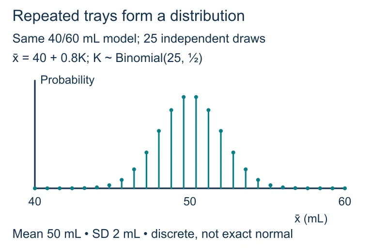Twenty-six possible sample means appear as discrete probability bars with a normal approximation drawn for comparison. For 25 independent fills equally likely to be 40 or 60 mL, K is binomial with n = 25 and p = 0.5, and the tray mean is 40 + 0.8K. The exact distribution is discrete, centered at 50 mL with standard deviation 2 mL. A normal curve approximates its shape.

SECTION 4

Mathematical Framework

The sampling distribution of x̄ is fully characterized by three properties: center, spread, and shape. Each property has a precise mathematical statement you must know for the AP exam.

CENTER (MEAN OF x̄)

μ_x̄ = μ

μ_x̄ is the mean of the sampling distribution; μ is the population mean. This holds for any sample size and any population shape.

SPREAD (STANDARD ERROR OF x̄)

σ_x̄ = σ / √n

σ is the population standard deviation; n is the sample size. This formula requires that observations are independent. When sampling without replacement, use the finite population correction factor √((N − n)/(N − 1)), but on the AP exam you may ignore it when n < 0.10N (the 10% condition).

SHAPE (CENTRAL LIMIT THEOREM)

x̄ ~ approximately N(μ, σ/√n) when n is sufficiently large

If the population itself is normal, then x̄ is exactly normal for every n. If the population is non-normal, the approximation improves as n increases. The traditional guideline is n ≥ 30 for moderately skewed populations; for strongly skewed or outlier-prone populations, larger n may be needed.

STANDARDIZATION (Z-SCORE FOR x̄)

z = (x̄ − μ) / (σ / √n)

This z-score tells you how many standard errors a particular sample mean is from the population mean. It is the basis for computing probabilities about x̄ using the standard normal table or a calculator's normalcdf function.

💡

AP Exam Tip — Conditions Checklist

Free-response questions typically require you to verify conditions before applying the normal model: (1) Random — the data come from a random sample or randomized experiment. (2) Independent — individual observations are independent; check the 10% condition when sampling without replacement. (3) Normal — the population is normal, or n is large enough for the CLT to apply. Failing to state these conditions will cost you rubric points.

SECTION 5

The Central Limit Theorem — A Closer Look

The Central Limit Theorem (CLT) is arguably the single most important theorem in introductory statistics. It guarantees that the distribution of x̄ converges to a normal distribution as n → ∞, no matter what the population distribution looks like — uniform, exponential, bimodal, or anything else. The rate of convergence depends on how far the population is from normality. A symmetric, unimodal population needs very few observations; a heavily skewed or multi-modal population requires more.

Three different population shapes (uniform, exponential, bimodal) produce sampling distributions that progressively approach normality. At n = 5, the uniform and bimodal populations already yield roughly normal x̄ distributions, while the exponential needs a larger sample. By n = 30, all three sampling distributions are approximately normal.

Population Shape	n needed for approximate normality of x̄	Guideline
Normal	Any n (exact normality)	No minimum required
Symmetric, no outliers	n ≥ 15	CLT kicks in quickly
Moderately skewed	n ≥ 30	Standard AP guideline
Strongly skewed or outlier-heavy	n ≥ 40 or more	Use caution; check graphical evidence

Sample-size guidelines for applying the Central Limit Theorem

SECTION 6

Worked Example — Computing a Probability About x̄

The daily caloric intake of adults in a large city has a mean of μ = 2200 calories and a standard deviation of σ = 400 calories. The distribution is right-skewed. A nutritionist selects a simple random sample of 50 adults. What is the probability that the sample mean caloric intake exceeds 2300 calories?

Finding P(x̄ > 2300)

1
Step 1 — Identify the Given Information

Population mean μ = 2200, population standard deviation σ = 400, sample size n = 50, and we want P(x̄ > 2300). The population is right-skewed.
2
Step 2 — Check Conditions

Random: The problem states a simple random sample. Independent: The city is large, so 50 < 10% of the population; the 10% condition is satisfied. Normal: n = 50 ≥ 30, so by the Central Limit Theorem, the sampling distribution of x̄ is approximately normal even though the population is right-skewed.

All three conditions are met ✓
3
Step 3 — Compute the Standard Error

σ_x̄ = σ / √n = 400 / √50 = 400 / 7.0711 ≈ 56.57 calories.

SE = 56.57 calories
4
Step 4 — Standardize (compute the z-score)

z = (x̄ − μ) / σ_x̄ = (2300 − 2200) / 56.57 = 100 / 56.57 ≈ 1.77.

z ≈ 1.77
5
Step 5 — Find the Probability

Using a standard normal table or the calculator command normalcdf(1.77, 1E99, 0, 1), we find P(Z > 1.77) ≈ 0.0384. Alternatively, normalcdf(2300, 1E99, 2200, 56.57) ≈ 0.0384.

P(x̄ > 2300) ≈ 0.0384, or about 3.84%
6
Step 6 — Interpret in Context

If we repeatedly draw random samples of 50 adults from this city, about 3.84% of those samples would have a mean caloric intake exceeding 2300 calories. This is a relatively unlikely outcome, suggesting that a sample mean of 2300 would be unusually high.

SECTION 7

Conditions, Common Pitfalls & Comparisons

Students frequently lose points on the AP exam because of predictable mistakes involving sampling distributions. The table below contrasts correct reasoning with the most common errors that graders see.

Topic	Correct Understanding	Common Mistake
Standard error vs. σ	σ_x̄ = σ/√n describes the variability of sample means, which is smaller than σ.	Using σ instead of σ/√n in the z-score denominator, which overstates the spread of x̄.
CLT vs. Law of Large Numbers	CLT describes the shape of the sampling distribution. LLN says x̄ converges to μ.	Confusing the two, or saying 'the CLT says x̄ gets closer to μ.'
Normality of x̄ vs. normality of population	The CLT makes x̄ approximately normal; it does NOT make the population normal or any individual sample normal.	Writing 'the CLT says the population is approximately normal for large n.'
10% condition	Required for independence when sampling without replacement: n < 0.10N.	Forgetting to check this condition or confusing it with the n ≥ 30 guideline for the CLT.
Known σ vs. estimated s	When σ is known, use z. When σ is unknown and estimated by s, use t.	Using a z-procedure when σ is unknown, or treating s and σ as interchangeable.

Common pitfalls involving sampling distributions of x̄

✦

KEY TAKEAWAY

The CLT is a statement about the distribution of x̄, not about the distribution of the original data. Just as a moving average in signal processing smooths out noise to reveal an underlying trend, increasing the sample size smooths out individual-level variability and makes the sampling distribution of the mean converge to a clean normal shape — but the raw population retains its original form.

SECTION 8

Connection to Inference & Advanced Topics

The sampling distribution of x̄ is not just an abstract concept — it is the engine that powers the two major inference procedures you will encounter later in the course: confidence intervals for μ and hypothesis tests about μ. Knowing that x̄ is approximately normal with mean μ and standard error σ/√n allows you to construct a z-interval (x̄ ± z* × σ/√n) when σ is known, or a t-interval (x̄ ± t* × s/√n) when it is not.

Feature	This Lesson (Known σ, z-model)	Next Steps (Unknown σ, t-model)
Parameter for spread	σ (population SD, known)	s (sample SD, estimated)
Standard error formula	σ / √n	s / √n
Reference distribution	Standard normal (z)	t-distribution with df = n − 1
Effect of small n	Still z, provided CLT or normality holds	Heavier tails to account for extra uncertainty in estimating σ
Practical frequency	Rare in practice (σ is seldom known)	Very common — the default one-sample t-procedure

From z-model (this lesson) to t-model (upcoming inference)

As you move through the inference unit, you will also encounter sampling distributions for differences of means (x̄₁ − x̄₂), which extend the same logic: the center is μ₁ − μ₂, the standard error is √(σ₁²/n₁ + σ₂²/n₂), and the shape is approximately normal by the CLT when both samples are large enough. Mastering the single-sample case in this lesson provides the template for all of these extensions.

SECTION 9

Practice Problems

Question 1: CONCEPTUAL

A population has a strongly left-skewed distribution with mean μ = 50 and standard deviation σ = 12. A researcher takes a simple random sample of size n = 64 and computes x̄. Which of the following best describes the sampling distribution of x̄?

A. Strongly left-skewed with mean 50 and standard deviation 12
B. Strongly left-skewed with mean 50 and standard deviation 1.5
C. Approximately normal with mean 50 and standard deviation 1.5
D. Approximately normal with mean 50 and standard deviation 12
E. Exactly normal with mean 50 and standard deviation 1.5

Show answer (C)

Correct answer: C. By the Central Limit Theorem, since n = 64 ≥ 30, the sampling distribution of x̄ is approximately normal with mean μ = 50 and standard error σ/√n = 12/√64 = 12/8 = 1.5. Choice A incorrectly keeps the population's skewed shape and uses σ instead of σ/√n. Choice B correctly computes the standard error but incorrectly retains the skewed shape. Choice D uses the population σ rather than the standard error. Choice E says 'exactly' normal, which is incorrect because the CLT provides only an approximation when the population is non-normal.

Question 2: BASIC CALCULATION

The weights of tomatoes at a farm are normally distributed with mean μ = 150 g and standard deviation σ = 20 g. If a random sample of 25 tomatoes is selected, what is the probability that the sample mean weight is less than 144 g?

A. 0.0013
B. 0.0228
C. 0.0668
D. 0.1587
E. 0.3821

Show answer (C)

Correct answer: C. Since the population is normal, x̄ is exactly normal: x̄ ~ N(150, 20/√25) = N(150, 4). The z-score is z = (144 − 150)/4 = −6/4 = −1.50. From the z-table, P(Z < −1.50) = 0.0668. Choice A (0.0013) corresponds to z ≈ −3.0, as if the standard error were not computed. Choice B (0.0228) corresponds to z = −2.0. Choice D (0.1587) corresponds to z = −1.0, which would result from using an incorrect standard error. Choice E (0.3821) corresponds to z ≈ −0.30, which is what you would get if you mistakenly used σ = 20 instead of σ/√n = 4.

Question 3: INTERMEDIATE

The mean commute time for employees at a large company is μ = 35 minutes with σ = 10 minutes. The distribution of individual commute times is right-skewed. A transportation analyst plans to sample commuters and compute x̄. For which of the following sample sizes would it be most reasonable to use a normal model for the sampling distribution of x̄?

A. n = 5
B. n = 10
C. n = 15
D. n = 20
E. n = 50

Show answer (E)

Correct answer: E. Because the population is described as right-skewed, we need a sufficiently large sample for the CLT to justify a normal approximation. The standard guideline for moderately skewed populations is n ≥ 30; for right-skewed distributions (which can be quite skewed when it comes to commute times that include outliers), n = 50 provides the strongest justification. Choices A, B, and C are all below the n ≥ 30 threshold, so a normal model would be questionable. Choice D (n = 20) is still below the guideline. Only n = 50 clearly satisfies the CLT condition for a right-skewed population.

Question 4: APPLIED

4 pts

A bottling plant fills juice bottles with a mean volume of μ = 500 mL and standard deviation σ = 8 mL. A quality inspector takes a random sample of 36 bottles each hour. In a given hour, the sample mean is x̄ = 497.5 mL. The inspector will flag the production line if the sample mean falls below 498 mL. (a) Verify that the conditions for using a normal model for the sampling distribution of x̄ are met. (b) What is the probability that x̄ falls below 498 mL when the process is operating correctly (μ = 500)? (c) In context, interpret the probability you computed in part (b). (d) The inspector observed x̄ = 497.5 mL. Based on your calculations, should the inspector be concerned? Explain using the sampling distribution.

Show answer

Rubric (4 points): Part (a) — Conditions (1 point): Random: The sample is described as random. Independent: 36 bottles is almost certainly less than 10% of all bottles produced in an hour at a bottling plant. Normal: n = 36 ≥ 30, so the CLT applies; alternatively, if the population is approximately normal, any n suffices. (Award 1 point for correctly checking all three conditions with justification.) Part (b) — Probability calculation (1 point): Standard error: σ/√n = 8/√36 = 8/6 ≈ 1.333 mL. z = (498 − 500)/1.333 = −2/1.333 ≈ −1.50. P(x̄ < 498) = P(Z < −1.50) ≈ 0.0668. (Award 1 point for correct standard error, z-score, and probability.) Part (c) — Interpretation in context (1 point): If the production process is operating correctly at μ = 500 mL, there is approximately a 6.68% probability that a random sample of 36 bottles would yield a sample mean below 498 mL. (Award 1 point for an interpretation that references the sampling process, includes the correct probability, and is stated in the context of juice bottle volumes.) Part (d) — Conclusion about x̄ = 497.5 (1 point): The observed x̄ = 497.5 corresponds to z = (497.5 − 500)/1.333 ≈ −1.875, giving P(x̄ < 497.5) ≈ 0.030. Since this is even further below 498 than the cutoff the inspector uses, and the probability of getting a sample mean this low (about 3%) is quite small if the process is on target, the inspector should be concerned. This provides evidence that the true mean may have shifted below 500 mL. (Award 1 point for correct reasoning connecting the observed value to the sampling distribution and providing a justified conclusion.)

Question 5: CRITICAL THINKING

4 pts

A researcher claims that for any population, the sampling distribution of x̄ is always approximately normal as long as the sample size is at least 30. (a) Explain why this claim is an oversimplification of the Central Limit Theorem. (b) Describe a specific type of population distribution for which n = 30 might not be sufficient to guarantee approximate normality of x̄. Justify your answer. (c) A study uses a random sample of size n = 10 from a population known to be normally distributed. Explain why the sampling distribution of x̄ is exactly normal in this case, and discuss whether the CLT is even needed. (d) Some textbooks state the CLT threshold as n ≥ 25 while others say n ≥ 30 or even n ≥ 40. Explain why there is no single universal threshold and what factors determine when the approximation is adequate.

Show answer

Rubric (4 points): Part (a) — Oversimplification (1 point): The CLT states that the sampling distribution of x̄ approaches normality as n increases, but the rate of convergence depends on the shape of the population distribution. For populations that are approximately symmetric and unimodal, n much smaller than 30 may suffice. For populations that are heavily skewed, have extreme outliers, or are multimodal, n = 30 may still produce a sampling distribution with noticeable non-normality. The number 30 is a rough guideline, not a mathematical boundary. (Award 1 point for clearly explaining that the n ≥ 30 rule is a guideline whose adequacy depends on population shape.) Part (b) — Problematic population (1 point): A population with a strongly right-skewed distribution, such as household income or insurance claims, could require n well above 30 because the long right tail means occasional very large values exert disproportionate influence on x̄. Similarly, a distribution with heavy tails (like a Cauchy distribution) may not satisfy the CLT at typical sample sizes because the variance is undefined or extremely large. (Award 1 point for identifying a specific type of distribution and justifying why n = 30 is insufficient.) Part (c) — Normal population with n = 10 (1 point): If the population is normally distributed, then any linear combination of normal random variables is also normal. Since x̄ = (1/n)ΣXᵢ is a linear combination of the n observations, x̄ is exactly normally distributed regardless of n. The CLT is not needed in this case; the result follows directly from the closure property of the normal distribution. (Award 1 point for correctly explaining that normality of x̄ follows from the normality of the population, not from the CLT.) Part (d) — No universal threshold (1 point): There is no single threshold because the CLT is an asymptotic result — it describes limiting behavior as n → ∞ — and different population distributions converge at different rates. The key factors are: (1) the degree of skewness — more skew requires larger n; (2) the presence and severity of outliers — heavy-tailed distributions converge more slowly; (3) the degree of multimodality — multiple modes can slow convergence. In practice, statisticians examine graphical displays (histograms, normal probability plots) of the sample data to assess whether the normal approximation for x̄ is reasonable for a given sample size. (Award 1 point for identifying at least two factors that influence the required sample size and explaining why no fixed number works universally.)

SUMMARY

Lesson Summary

Summary

The sampling distribution of the sample mean describes the behavior of x̄ across all possible random samples of size n from a population. Its center is μ (making x̄ an unbiased estimator), its spread is σ/√n (the standard error, which shrinks as n increases), and its shape becomes approximately normal by the Central Limit Theorem when n is sufficiently large — typically n ≥ 30 for skewed populations, though smaller n works for populations that are already close to normal.

To apply these results on the AP exam, always verify the Random, Independent (10% condition), and Normal/Large Sample conditions. Use z = (x̄ − μ) / (σ/√n) to standardize x̄ and find probabilities. Remember that the CLT describes the distribution of the statistic x̄, not the population itself. This foundational concept extends directly to confidence intervals and hypothesis tests for population means, forming the backbone of statistical inference.