Random Sampling and Data Collection - AP Statistics

SECTION 1

Historical Context & Motivation

Statistical thinking has always been motivated by a deceptively simple question: how can we learn about a large group by examining only a small part of it? For centuries, governments conducted full censuses—counting every individual—but the cost and logistical burden of such efforts drove mathematicians and social scientists to develop sampling methods that could produce reliable conclusions from partial data. The intellectual leap from enumeration to inference depended on a single breakthrough idea: randomness as a deliberate tool for fairness. Without randomness, samples can systematically over-represent or under-represent segments of a population, producing conclusions that are not just imprecise but fundamentally misleading.

1895 • Anders Kiaer's Representative Method

Norwegian statistician Anders Kiaer proposed purposive sampling for social surveys at the International Statistical Institute, sparking decades of debate about whether deliberately chosen samples could represent whole populations.

1934 • Jerzy Neyman's Landmark Paper

Neyman demonstrated mathematically that probability-based sampling allows valid estimation of sampling error, establishing the theoretical foundation for modern random sampling and stratified designs.

1936 • The Literary Digest Debacle

The Literary Digest polled 2.4 million people but predicted the wrong winner in the U.S. presidential election, while George Gallup's smaller random sample predicted correctly—proving that sample quality trumps sample size.

1940s • Rise of Modern Survey Sampling

The U.S. Census Bureau and academic researchers adopted probability sampling frameworks for government surveys and social research, making random sampling the gold standard for data collection worldwide.

2000s–Present • Digital-Age Sampling Challenges

The explosion of online data introduced new forms of convenience and voluntary response sampling, renewing focus on the foundational importance of probability-based methods for valid inference.

The 1936 Literary Digest disaster remains the most cited cautionary tale in statistics: a massive sample drawn from telephone directories and automobile registrations over-represented wealthier voters, producing a prediction that was spectacularly wrong. Meanwhile, George Gallup's far smaller but carefully randomized sample produced an accurate forecast. The lesson crystallized what Neyman had proven theoretically—how you select your sample matters far more than how large it is. This section of the AP Statistics curriculum asks you to master the principles that make data collection valid, recognizing that every confidence interval, hypothesis test, and regression model you will ever build depends on the integrity of the data feeding it.

SECTION 2

Core Principles & Definitions

Before examining specific sampling techniques, you need a precise vocabulary. A population is the entire group of individuals or objects about which you want information—every registered voter, every light bulb produced on a factory line, every white-tailed deer in a national forest. A sample is the subset of the population that you actually observe. The goal of statistical sampling is to use information from the sample to draw conclusions—inferences—about the population. The critical question is whether those inferences are trustworthy, and the answer depends almost entirely on how the sample was selected.

Random Selection

Every member of the population has a known, non-zero probability of being selected. This is the defining feature of probability sampling and the basis for computing margins of error.

Bias vs. Variability

Bias is the systematic tendency to over- or under-estimate a population parameter. Variability describes how much the statistic would change from sample to sample. Increasing sample size reduces variability but does NOT fix bias.

Sampling Frame

The sampling frame is the list of individuals from which the sample is actually drawn. When the frame does not match the population (undercoverage), bias is introduced regardless of how random the selection process is.

Generalizability

Results from a random sample can be generalized to the population from which it was drawn. Without random selection, you can describe the sample but cannot make valid inferences about any larger group.

Sources of Bias

Common sources include voluntary response bias (only passionate individuals respond), nonresponse bias (selected individuals refuse to participate), and response bias (wording or context distorts answers).

✦

KEY TAKEAWAY

Think of random sampling like shuffling a deck of cards before dealing. If you shuffle properly, every card has an equal chance of appearing in any position, so the hand you receive is a fair representation of the full deck. If you skip the shuffle and deal from the top of a sorted deck, your hand is systematically unrepresentative—no matter how many cards you deal. In statistics, randomness is the shuffle that prevents systematic distortion.

SECTION 3

Visual Explanation — Sampling Methods Overview

The diagram below illustrates the four major probability sampling methods you must know for the AP Statistics exam. Each method uses randomness differently to select individuals from a population, and each has distinct advantages depending on the structure of the population and the practical constraints of the study.

The top row shows the four probability sampling methods (colored dots indicate selected individuals). The bottom panel contrasts these with three common non-probability methods that introduce systematic bias.

Notice the fundamental distinction among the probability methods. In a simple random sample, every possible sample of size n has an equal chance of being chosen—this is the purest form of random selection. Stratified random sampling first classifies the population into non-overlapping subgroups (strata) based on a characteristic expected to influence the response, then draws a separate SRS from each stratum—this guarantees representation from every group and typically reduces variability. Cluster sampling randomly selects entire groups (clusters) and then surveys every individual within the chosen clusters—this is practical when a complete list of individuals is unavailable but a list of clusters is. Systematic sampling selects a random starting point and then picks every kth individual from an ordered list, which is efficient but can be biased if the list has a periodic pattern aligned with k.

A university campus provides a setting for comparing sampling and study-design routes. The way people or groups enter a study determines its design. Sampling within groups, selecting whole groups and assigning treatments answer different questions.

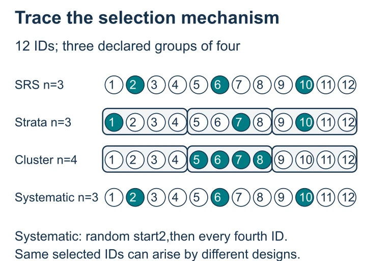Four 12-ID diagrams show a simple random sample, one selection from each stratum, all members of one cluster and a systematic sequence. The 12-ID examples use different selection rules: an SRS selects from the whole list; stratification selects within every group; cluster sampling takes all IDs in the chosen group; systematic sampling uses a random start and fixed spacing. The selection rule, not a single realized sample, identifies the design.

SECTION 4

Mathematical Framework

While the AP Statistics exam does not require you to derive sampling distributions from first principles, understanding the mathematical relationships between sample size, variability, and margin of error gives you the conceptual foundation for the inference procedures you will encounter throughout the course. The formulas below connect the mechanics of random sampling to the quantitative measures of precision that make statistical inference possible.

MARGIN OF ERROR (PROPORTIONS)

ME = z* × √( p̂(1 − p̂) / n )

where z* is the critical value for the desired confidence level, p̂ is the sample proportion, and n is the sample size. Notice that the margin of error decreases with the square root of n—quadrupling the sample size halves the margin of error.

SELECTION PROBABILITY (SRS)

P(individual i selected) = n / N

In a simple random sample of size n from a population of size N, every individual has the same probability of being included. This equal probability is what allows us to compute unbiased estimators of population parameters.

SYSTEMATIC SAMPLING INTERVAL

k = N / n

Choose a random starting point between 1 and k, then select every kth individual. For example, from a population of N = 5000, a sample of n = 100 requires k = 50, so you might start at individual 23 and then select 73, 123, 173, and so on.

NUMBER OF POSSIBLE SRS SAMPLES

C(N, n) = N! / (n!(N − n)!)

The combination formula gives the total number of distinct samples of size n from a population of size N. An SRS ensures each of these C(N, n) samples is equally likely. Even for modest populations, this number is astronomically large, which is why random selection is so powerful: bias would require systematically avoiding certain combinations.

📐

WHY SAMPLE SIZE MATTERS (BUT NOT AS MUCH AS YOU THINK)

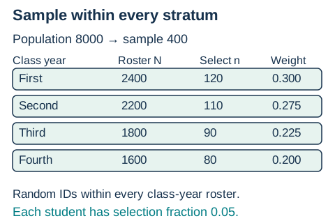The margin of error formula reveals a square-root relationship: to cut your margin of error in half, you need to multiply your sample size by four. This diminishing return is why national polls of 1,000–1,500 randomly selected adults can estimate opinions for 330 million people with a margin of error of about ±3 percentage points. The precision depends on the absolute size of the sample, not on the fraction of the population sampled—a counterintuitive but mathematically provable fact.

Four rows list class-year populations 2,400, 2,200, 1,800 and 1,600; selected samples 120, 110, 90 and 80; and weights 0.300, 0.275, 0.225 and 0.200. For a university with 8,000 students, allocate 400 selections as 120, 110, 90 and 80 across the four class-year rosters, then choose random IDs within each roster. Each student has a 5% selection chance; the fixed class-year allocations make this a stratified sample, not an SRS of 400.Open full diagram

SECTION 5

Sources of Bias in Data Collection

Even a well-designed sampling plan can be undermined by bias that creeps in during the data-collection process. The AP Statistics exam frequently tests your ability to identify and distinguish among several types of bias. The diagram below organizes these sources into a decision flowchart that traces where in the sampling pipeline each type of bias can occur.

This pipeline shows that bias can enter at multiple stages of data collection. Random sampling directly addresses selection bias, but researchers must also guard against undercoverage, nonresponse, voluntary response, response, and measurement bias.

Type of Bias	Definition	Classic Example
Undercoverage	Some members of the population are left out of the sampling frame	Phone survey using landlines only excludes cell-phone-only households
Voluntary Response	Individuals self-select into the sample, typically those with strong opinions	Online product reviews skew negative because dissatisfied customers are more motivated to post
Nonresponse	Selected individuals cannot be contacted or refuse to participate	Mailed health survey has 20% response rate; respondents may be healthier than non-respondents
Response Bias	Respondents give inaccurate answers due to question wording, interviewer influence, or social desirability	Asking "Don't you agree that..." leads respondents toward a particular answer
Convenience Sampling	Researcher selects whoever is most accessible, with no randomization	Surveying students in the library about study habits over-represents studious individuals

Common sources of bias tested on the AP Statistics exam

💡

AP Exam Tip

When a free-response question asks you to identify a source of bias, do three things: (1) name the bias, (2) explain the mechanism by which it operates in the given context, and (3) state the direction of the bias (does it tend to overestimate or underestimate the parameter of interest?). Simply naming the bias without explaining the direction typically earns only partial credit.

SECTION 6

Worked Example — Designing a Sampling Plan

A school district with 12 elementary schools (total enrollment 4,800 students) wants to estimate the proportion of students who eat breakfast every morning. The district has a complete roster of all students organized by school. Design a stratified random sampling plan and explain why it is preferable to a simple random sample in this context.

Designing a Stratified Random Sample

1
Step 1 — Identify the Population and Parameter

The population is all 4,800 elementary students in the district. The parameter of interest is p, the true proportion of students who eat breakfast every morning.

Population: 4,800 students across 12 schools
2
Step 2 — Define the Strata

Because breakfast habits may vary by school (due to differences in socioeconomic composition, proximity to restaurants, or school breakfast programs), we use each of the 12 schools as a stratum. This ensures that every school is represented in the final sample and reduces variability by accounting for school-to-school differences.

12 strata, one per school
3
Step 3 — Determine Sample Size and Allocation

Suppose we want a total sample of n = 240 students (5% of the population). Using proportional allocation, each school contributes students in proportion to its enrollment. For example, a school with 600 students (600/4800 = 12.5% of the population) contributes 0.125 × 240 = 30 students to the sample.

n = 240 total; proportional allocation per school
4
Step 4 — Random Selection Within Each Stratum

Within each school, assign every student a number (e.g., 001–600 for the school above). Use a random number generator or a table of random digits to select the required number of students. Each student within a school has an equal probability of being selected. This process is repeated independently for each of the 12 schools.

SRS within each stratum using random number generator
5
Step 5 — Justify the Method Over SRS

A simple random sample of 240 from 4,800 might, by chance, over-represent some schools and miss others entirely. By stratifying, we guarantee representation from every school and reduce the variability of our estimate because within-school variability in breakfast habits is likely smaller than between-school variability. The result is a more precise estimate of the district-wide proportion for the same sample size.

Stratified sampling is more precise because it ensures representation and exploits within-stratum homogeneity.

SECTION 7

Comparing Sampling Methods — Strengths & Limitations

Each sampling method involves tradeoffs between statistical precision, practical feasibility, and cost. The table below summarizes the strengths and limitations you should be prepared to discuss on the AP exam. Understanding these tradeoffs is essential for free-response questions that ask you to select and justify a sampling design for a given scenario.

Method	Strengths	Limitations
Simple Random Sample (SRS)	Eliminates selection bias; every sample of size n equally likely; simplest to analyze; foundation for all other methods	Requires a complete list of the population; may be impractical for geographically dispersed populations; can miss small subgroups by chance
Stratified Random Sample	Guarantees representation of all subgroups; typically more precise than SRS for the same n; allows separate analysis of each stratum	Requires advance knowledge of a relevant stratifying variable; requires a complete list within each stratum; more complex to administer
Cluster Sample	Does not require a list of every individual—only a list of clusters; cost-effective for geographically spread populations; practical for large-scale studies	Higher variability than SRS or stratified for the same n; biased if clusters are not representative; selected clusters may share unique characteristics
Systematic Sample	Easy to implement; spreads sample evenly across the ordered list; does not require labeling every individual in advance	Biased if the list has a periodic pattern matching k; technically not an SRS (not every combination of n individuals is equally likely)

Comparison of the four probability sampling methods

⚡

STRATIFIED ≠ CLUSTER — A CRITICAL DISTINCTION

Students frequently confuse stratified and cluster sampling because both involve dividing the population into groups. The key difference lies in what you do after forming the groups. In stratified sampling, you sample from every group (you want representation from each stratum). In cluster sampling, you randomly select some groups and skip others (then survey everyone in the chosen clusters). Think of it this way: strata should be internally homogeneous but different from each other (like sorting M&Ms by color and grabbing some of each), while clusters should each be a mini-replica of the whole population (like scooping a handful from one bag and hoping it represents all the bags).

SECTION 8

Connection to Statistical Inference

Everything you learn about random sampling in Unit 4 of AP Statistics exists to support the inference procedures you will encounter in Units 6–9. The connection is direct: confidence intervals and hypothesis tests are valid only when the data come from a well-designed random sample or randomized experiment. Without random selection, the sampling distribution—the theoretical framework that underlies every p-value and confidence interval—does not apply, and your conclusions have no guaranteed connection to the population.

Data Collection Concept	Inference Consequence
Random sampling from population	Results can be generalized to the entire population from which the sample was drawn
Random assignment to treatments	Cause-and-effect conclusions can be drawn about the treatments
Both random sampling AND random assignment	Causal conclusions can be generalized to the population—the gold standard
Neither random sampling nor random assignment	No generalization and no causal claims—only associations within the observed sample

The Scope of Conclusions framework — essential for AP exam free-response

This framework is sometimes called the Scope of Conclusions table, and it appears frequently on AP free-response questions. When you write conclusions for inference problems, your language must match the study design. If a study used random sampling but not random assignment, you may generalize to the population (e.g., "we can estimate the proportion of all students who...") but you may not claim causation. Conversely, an experiment with random assignment but convenience sampling can establish causation within the sample but cannot generalize to a broader population.

ℹ

Looking Ahead

In Unit 5 (Probability) you will formalize the notion of a sampling distribution—the distribution of a statistic across all possible random samples of size n. The conditions for applying inference procedures (randomness, independence, normality) all trace back to whether the data were collected using proper random sampling or random assignment. Master the data collection principles now, and the logic of inference will follow naturally.

SECTION 9

Practice Problems

Question 1: CONCEPTUAL

A researcher wants to estimate the average commute time for employees at a large company with 5,000 workers. She posts a survey on the company intranet and receives 800 responses. Which of the following best describes a potential problem with this sampling method?

A. The sample size of 800 is too small relative to the population of 5,000.
B. The sample may suffer from voluntary response bias because employees choose whether to respond, and those with extreme commute times may be more motivated to participate.
C. The sampling frame does not match the population because not all employees have internet access.
D. The researcher should have used a census instead of a sample.
E. The results cannot be analyzed because the sample was not stratified by department.

Show answer (B)

Correct answer: B. This is a voluntary response sample because employees self-select into the survey. People with unusually long or short commutes—or those with strong feelings about commuting—are more likely to respond, systematically skewing the results. A is incorrect because 800 out of 5,000 (16%) is a large sample; the issue is not size but the method of selection. C is incorrect because a company intranet is typically accessible to all employees; while undercoverage is possible, the primary concern here is self-selection. D is incorrect because a census is not required—a well-designed random sample would suffice. E is incorrect because stratification is a design improvement, not a requirement for analysis; the fundamental problem is the lack of random selection.

Question 2: BASIC CALCULATION

A factory produces 10,000 widgets per day. A quality-control manager wants to select a systematic sample of 200 widgets. She will randomly select a starting point and then choose every kth widget. What is the value of k?

A. 20
B. 50
C. 100
D. 200
E. 500

Show answer (B)

Correct answer: B. The sampling interval for a systematic sample is k = N/n = 10,000/200 = 50. The manager randomly selects a starting widget between 1 and 50 (say, widget 17), then selects every 50th widget after that: 17, 67, 117, 167, and so on. A (k = 20) would give n = 10,000/20 = 500 widgets, which is too many. C (k = 100) yields only n = 100. D (k = 200) confuses the sample size with the interval. E (k = 500) would produce only 20 widgets. Always use k = N/n and verify that selecting every kth item gives you exactly n items.

Question 3: INTERMEDIATE

A state education agency wants to estimate the average reading score of all fourth-graders in the state. They randomly select 40 schools from a list of all elementary schools in the state, and then test every fourth-grader in each selected school. Which sampling method is being used, and what is a potential drawback?

A. Stratified random sample; a drawback is that it requires a complete list of all fourth-graders.
B. Simple random sample; a drawback is that some schools may be over-represented.
C. Cluster sample; a drawback is that schools selected by chance may not represent the full diversity of schools in the state, increasing variability.
D. Systematic sample; a drawback is that periodic patterns in the school list could introduce bias.
E. Convenience sample; a drawback is that the agency chose schools that were easy to access.

Show answer (C)

Correct answer: C. This is a cluster sample because the agency randomly selected whole schools (clusters) and then tested all fourth-graders within those schools. The primary drawback is that cluster sampling generally has higher variability than SRS or stratified sampling for the same total sample size, because students within a single school tend to be more similar to each other than to students at other schools. If the 40 selected schools happen to be disproportionately urban or rural, the estimate will be less precise. A is incorrect because in a stratified sample, every stratum contributes to the sample—here, most schools are excluded. B is incorrect because individuals were not independently selected—they were included because their school was chosen. D is incorrect because there is no kth-item selection rule. E is incorrect because the schools were randomly selected, not chosen for convenience.

Question 4: APPLIED

4 pts

A university dining services director wants to estimate the proportion of students who are satisfied with the campus meal plan. The university has 8,000 undergraduates: 2,400 freshmen, 2,200 sophomores, 1,800 juniors, and 1,600 seniors. The director decides to use a stratified random sample of 400 students, with class year as the stratifying variable. (a) Explain why stratifying by class year is a reasonable choice in this context. (b) Calculate how many students should be sampled from each class year using proportional allocation. (c) Describe the process for selecting the freshmen in the sample. Be specific enough that another researcher could replicate the procedure. (d) A friend suggests it would be easier to just hand surveys to students leaving the dining hall during lunch. Identify the sampling method the friend is proposing, name one likely source of bias, and explain the direction of that bias.

Show answer

Part (a) — 1 point: Satisfaction with the meal plan is likely to vary by class year because freshmen are often required to purchase a meal plan while upperclassmen may have more dining options. Stratifying by class year ensures that each year is proportionally represented in the sample and reduces variability by grouping students who may have similar dining experiences together. Part (b) — 1 point: The sampling fraction is 400/8,000 = 0.05. Freshmen: 2,400 × 0.05 = 120. Sophomores: 2,200 × 0.05 = 110. Juniors: 1,800 × 0.05 = 90. Seniors: 1,600 × 0.05 = 80. Total: 120 + 110 + 90 + 80 = 400. ✓ Part (c) — 1 point: Obtain a complete list of all 2,400 freshmen from the registrar. Assign each freshman a unique number from 0001 to 2400. Using a random number generator (or a table of random digits reading four-digit numbers), generate numbers between 0001 and 2400, skipping duplicates and numbers outside this range. Continue until 120 unique freshmen have been selected. Contact each selected student to administer the survey. Part (d) — 1 point: The friend's method is a convenience sample. A likely source of bias is that students who eat at the dining hall during lunch are more likely to be regular meal-plan users and therefore potentially more satisfied with the plan than students who avoid the dining hall. This would produce an overestimate of the true proportion of students who are satisfied with the meal plan.

Question 5: CRITICAL THINKING

4 pts

A national health organization conducts a telephone survey to estimate the percentage of adults who exercise at least 150 minutes per week. The organization uses random digit dialing to select a simple random sample of 2,000 phone numbers, but only 650 people agree to complete the survey. (a) The organization claims the results can be generalized to all U.S. adults because the initial selection was random. Critique this claim. (b) Suppose the people who agreed to respond exercise, on average, more than those who refused. Explain how this would affect the estimate and identify the specific type of bias at work. (c) Propose two specific strategies the organization could use to reduce the bias you identified in part (b). Explain why each strategy would help. (d) Even if the organization achieves a 100% response rate, explain one additional source of bias that could still affect the results and state its likely direction.

Show answer

Part (a) — 1 point: The claim is flawed because the initial random selection only ensures that the 2,000 phone numbers are representative. However, only 650 of the 2,000 selected individuals actually responded, giving a response rate of only 32.5%. If the 1,350 non-respondents differ systematically from the 650 respondents with respect to exercise habits—which is highly plausible—then the final sample of 650 is no longer representative of the population. Random selection of the initial sample does not compensate for severe nonresponse. Part (b) — 1 point: If respondents exercise more than non-respondents on average, the survey will overestimate the true percentage of adults who exercise at least 150 minutes per week. This is nonresponse bias: the individuals who were selected but did not respond have different characteristics (lower exercise levels) than those who did respond, and their absence from the data systematically tilts the estimate upward. Part (c) — 1 point: Strategy 1: Implement multiple follow-up contact attempts (calling back at different times of day and on different days of the week). This would help because many non-respondents may simply have been unavailable rather than unwilling, and reaching them would make the responding sample more representative. Strategy 2: Offer incentives for participation (e.g., a gift card or small payment). This reduces nonresponse by motivating people who might otherwise decline, including those who exercise less and may have weaker intrinsic motivation to discuss health behaviors. Part (d) — 1 point: Response bias (specifically, social desirability bias) could still affect the results. Respondents may overreport their exercise levels because they perceive regular exercise as socially valued behavior, especially when speaking to a human interviewer. This would cause the survey to overestimate the true percentage of adults meeting the 150-minute threshold, even with a 100% response rate.

SUMMARY

Random Sampling and Data Collection — Summary

Summary

Valid statistical inference begins with proper data collection. Random sampling ensures that every member of the population has a known, non-zero chance of selection, which eliminates selection bias and provides the mathematical foundation for computing margins of error and constructing confidence intervals. The four probability sampling methods—simple random, stratified random, cluster, and systematic—each use randomness in a different way and offer distinct tradeoffs between precision, cost, and practicality.

Beyond the selection mechanism, you must be vigilant about sources of bias that can corrupt data at every stage of the collection pipeline: undercoverage when the sampling frame misses population members, nonresponse bias when selected individuals fail to participate, voluntary response bias when individuals self-select, and response bias when question wording or social desirability distorts answers. Remember the Scope of Conclusions framework: random sampling allows generalization to the population, random assignment allows causal claims, and you need both for generalizable causal conclusions. Increasing sample size reduces variability but never fixes bias—only sound design can do that.