Mean and Standard Deviation of Random Variables - AP Statistics

SECTION 1

Historical Context & Motivation

Long before modern statistics formalized the language of random variables, mathematicians and gamblers were grappling with a fundamental question: if a random process is repeated many times, what outcome should one expect on average, and how much will individual outcomes deviate from that average? This twin concern—center and spread—drove centuries of mathematical innovation. The concept of the expected value emerged from correspondence among European mathematicians debating the fair price of games of chance, while the notion of standard deviation crystallized much later as astronomers sought to quantify the reliability of their measurements.

1654 • Pascal–Fermat Correspondence

Blaise Pascal and Pierre de Fermat exchanged letters on the "problem of points," laying the groundwork for probability theory and the idea that uncertain outcomes have a calculable long-run average.

1657 • Huygens and Expected Value

Christiaan Huygens published De Ratiociniis in Ludo Aleae, introducing what would become the concept of expected value—the probability-weighted average of all possible outcomes.

1713 • Bernoulli's Ars Conjectandi

Jacob Bernoulli's posthumous masterwork proved the Law of Large Numbers, demonstrating that sample means converge to the expected value as the number of trials grows.

1893 • Pearson Coins "Standard Deviation"

Karl Pearson introduced the term "standard deviation" as a measure of dispersion, replacing various inconsistent notations and formalizing the concept for modern statistics.

Today, the mean (expected value) and standard deviation of a random variable form the twin pillars on which probability distributions rest. Together they answer two essential questions: Where is the distribution centered? and How much variability exists around that center? Understanding these parameters is essential for everything from insurance pricing to quality control in manufacturing, and they appear throughout the AP Statistics curriculum.

SECTION 2

Core Principles & Definitions

A random variable assigns a numerical value to each outcome of a random process. When we describe its probability distribution—the complete list of values and their associated probabilities—we can compute summary measures that characterize the distribution's behavior. The mean and standard deviation are the two most important of these measures, and they parallel the sample mean (x̄) and sample standard deviation (s) you already know from descriptive statistics, but they describe the theoretical population of all possible outcomes rather than a finite dataset.

Mean (Expected Value) μ_X

The probability-weighted average of all possible values of the random variable. It represents the long-run average outcome if the random process were repeated indefinitely. Denoted μ_X or E(X).

Variance σ²_X

The probability-weighted average of the squared deviations from the mean. Variance measures spread in squared units, making it useful for algebraic manipulation but less interpretable on its own.

Standard Deviation σ_X

The positive square root of the variance. It returns the measure of spread to the original units of the random variable, making it directly interpretable as a typical deviation from the mean.

Discrete vs. Continuous

For discrete random variables, summation (Σ) is used. For continuous random variables, integration (∫) replaces summation. On the AP exam, you work primarily with discrete distributions and named continuous distributions.

✦

KEY TAKEAWAY

Think of the mean μ_X as the balance point of the probability distribution—just as a physical seesaw balances where the weighted masses on each side are equal. The standard deviation σ_X then measures how far, on average, the outcomes sit from that balance point. In engineering and finance, these two numbers together tell you the expected performance of a system and how much risk surrounds that expectation.

SECTION 3

Visualizing the Mean and Standard Deviation

The following diagram illustrates the probability distribution of a discrete random variable X representing the number of heads in three fair coin flips. The probability histogram shows all possible values (0, 1, 2, 3), their probabilities, the location of the mean μ_X = 1.5, and the interval within one standard deviation of the mean.

The dashed pink line marks the mean μ_X = 1.5, which is the balance point of the distribution. The shaded violet region shows the interval from μ − σ to μ + σ (approximately 0.63 to 2.37). Notice that the values x = 1 and x = 2, which together carry 75% of the total probability, fall within this one-standard-deviation band.

Several features of this diagram are worth noting. First, the mean μ_X = 1.5 does not correspond to any value that X can actually take—it is a theoretical long-run average, not a possible outcome. Second, the distribution is symmetric, so the mean falls exactly at the midpoint. Third, the standard deviation σ_X ≈ 0.87 captures the fact that most of the probability mass is concentrated near the center; if the distribution were more spread out (e.g., all four values equally likely), the standard deviation would be larger.

SECTION 4

Mathematical Framework

The formulas for the mean and standard deviation of a discrete random variable follow directly from the idea of probability-weighted averaging. Unlike descriptive statistics where each data point is counted equally, here each value is weighted by its probability of occurring. This section presents the three core formulas you must know for the AP exam, along with the rules for linear transformations and combinations of random variables.

MEAN (EXPECTED VALUE)

μ_X = E(X) = Σ x_i · P(x_i)

Sum over all possible values x_i of the random variable. Each value is multiplied by its probability P(x_i), and the products are summed.

VARIANCE

σ²_X = Var(X) = Σ (x_i − μ_X)² · P(x_i)

Each squared deviation (x_i − μ_X)² is weighted by its probability. The result is in squared units of X.

STANDARD DEVIATION

σ_X = √(σ²_X) = √[ Σ (x_i − μ_X)² · P(x_i) ]

Taking the square root returns the spread measure to the original units of X, making it directly interpretable.

Rules for Linear Transformations

If Y = a + bX, where a and b are constants, then the mean and standard deviation transform predictably. The linear transformation rules state that μ_Y = a + bμ_X and σ_Y = |b| × σ_X. Adding a constant shifts the mean but does not affect the spread. Multiplying by a constant scales both the mean and the standard deviation.

COMBINING INDEPENDENT RANDOM VARIABLES

μ_{X±Y} = μ_X ± μ_Y σ²_{X±Y} = σ²_X + σ²_Y

For independent random variables X and Y: means add or subtract as expected, but variances always ADD—even when subtracting the random variables. Standard deviations do NOT add directly.

⚠

AP Exam Alert

A common exam trap: when computing the spread of X − Y for independent variables, students mistakenly subtract the variances. Remember, variances always add when combining independent random variables, whether you are adding or subtracting them. The difference of two independent random variables is more variable than either one alone.

SECTION 5

Transformations & Combinations in Detail

Understanding how the mean and standard deviation behave under transformations and combinations is one of the most tested skills on the AP Statistics exam. The diagram below provides a visual summary of the key rules, illustrating how shifting, scaling, and combining independent random variables affect the center and spread of a distribution.

A summary of all transformation and combination rules for random variables. The violet and amber boxes cover single-variable transformations. The emerald and red boxes cover combining two independent random variables. Note particularly that the red box (difference) still shows variances adding—this is the most commonly tested point.

A critical distinction worth reinforcing: the combination rules for variance require independence. If X and Y are not independent, you must account for their covariance, and the variance formula becomes σ²_X±Y = σ²_X + σ²_Y ± 2Cov(X, Y). On the AP exam, however, you will almost always be told that the variables are independent, which simplifies the formula by setting the covariance term to zero. Always check the problem statement for this condition before applying the rules.

💡

Why Variances Add When Subtracting

Imagine independently choosing a random person's height in the U.S. and a random person's height in Japan, then computing the difference. The difference is uncertain because both selections inject randomness into the result. Whether you add or subtract two independent sources of uncertainty, the total uncertainty (variance) increases.

SECTION 6

Worked Example

A small insurance company sells a one-year policy that pays out $10,000 with probability 0.02 and $0 otherwise. The annual premium is $300. Let X represent the company's profit on a randomly selected policy. Find the mean and standard deviation of X.

Insurance Policy Profit

1
Step 1 — Define the Random Variable and Its Distribution

The profit X depends on whether the company pays a claim. If no claim is filed (probability 0.98), the company keeps the $300 premium, so X = $300. If a claim is filed (probability 0.02), the company receives $300 in premium but pays $10,000, so X = $300 − $10,000 = −$9,700.
2
Step 2 — Set Up the Probability Distribution Table

X takes two values: x₁ = 300 with P(x₁) = 0.98, and x₂ = −9,700 with P(x₂) = 0.02. Verify that probabilities sum to 1: 0.98 + 0.02 = 1 ✓.
3
Step 3 — Compute the Mean

μ_X = Σ x_i × P(x_i) = (300)(0.98) + (−9,700)(0.02) = 294 + (−194) = 100.

μ_X = $100
4
Step 4 — Compute the Variance

σ²_X = Σ (x_i − μ_X)² × P(x_i) = (300 − 100)²(0.98) + (−9,700 − 100)²(0.02) = (200)²(0.98) + (−9,800)²(0.02) = 40,000(0.98) + 96,040,000(0.02) = 39,200 + 1,920,800 = 1,960,000.

σ²_X = 1,960,000 dollars²
5
Step 5 — Compute the Standard Deviation

σ_X = √1,960,000 = 1,400.

σ_X = $1,400
6
Step 6 — Interpret in Context

On average, the company expects to profit $100 per policy sold. However, the standard deviation of $1,400 indicates enormous variability in individual policy outcomes—the profit from any single policy is highly unpredictable. This is why insurance companies sell many policies: the Law of Large Numbers ensures the average profit per policy approaches μ_X = $100 as the number of policies grows.

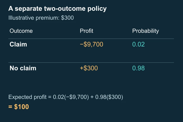
A separate $300-premium, two-outcome insurance distribution: profits −9700 and 300 with probabilities 0.02 and 0.98, giving expected profit 100.

$300 premium, two-outcome distribution.

SECTION 7

Mean vs. Standard Deviation: Strengths & Limitations

The mean and standard deviation each capture a distinct aspect of a random variable's probability distribution, and each has strengths and limitations that determine when it is most useful. Comparing them side by side clarifies their complementary roles.

Feature	Mean (μ_X)	Standard Deviation (σ_X)
Measures	Center / long-run average	Spread / typical deviation from center
Units	Same as X	Same as X (variance is in squared units)
Affected by outliers?	Yes—extreme values with even small probabilities can shift the mean	Yes—extreme values inflate squared deviations substantially
Additive for independent RVs?	Means always add (no independence needed)	Standard deviations do NOT add; variances add only for independent RVs
Key limitation	Tells nothing about shape or spread of the distribution	Tells nothing about center; alone cannot determine shape

Comparison of mean and standard deviation as summary measures of a random variable's distribution.

✦

KEY TAKEAWAY

Neither the mean nor the standard deviation alone fully describes a distribution. In practice—whether in pharmaceutical trials assessing the expected efficacy of a drug (mean) and the patient-to-patient variability in response (standard deviation), or in portfolio theory balancing expected returns against risk—you need both parameters working together. On the AP exam, always report both center and spread when describing a distribution, and interpret them in context.

SECTION 8

Connections to Advanced Theory

The mean and standard deviation of random variables are not isolated topics; they form the theoretical foundation for several major ideas that appear later in the AP Statistics curriculum and in college-level probability. The table below connects the concepts from this lesson to the broader statistical framework.

This Lesson	Advanced Extension	Connection
μ_X = Σ $x_i$ · P( $x_i$ )	Sampling distributions: μ_x̄ = μ	The mean of the sampling distribution equals the population mean—an unbiased estimator result.
σ²_{X+Y} = σ²_X + σ²_Y	Sampling distributions: σ_x̄ = σ / √n	The variance-addition rule applied n times leads to the formula for the standard error of the sample mean.
Linear transformation rules	Z-scores: Z = (X − μ) / σ	Standardization is a linear transformation that produces μ_Z = 0 and σ_Z = 1.
Expected value E(X)	Binomial: μ = np, σ = √(np(1−p))	The binomial formulas are derived by summing n independent Bernoulli random variables using the combination rules from this lesson.

How the mean and standard deviation of random variables connect to topics later in the AP Statistics course.

Perhaps the most powerful downstream application is the Central Limit Theorem, which states that the sampling distribution of the sample mean x̄ is approximately normal for large n, with mean μ and standard deviation σ/√n. This theorem relies entirely on the concepts of expected value and variance addition for independent random variables. When you encounter confidence intervals and hypothesis tests later in the course, remember that the machinery powering those procedures was built from the rules you learned here—specifically, how means and variances combine when independent random variables are summed.

SECTION 9

Practice Problems

Question 1: CONCEPTUAL

A discrete random variable X has mean μ_X = 5 and standard deviation σ_X = 2. A new random variable Y is defined as Y = 3X − 4. What are the mean and standard deviation of Y?

A. μ_Y = 11, σ_Y = 2
B. μ_Y = 15, σ_Y = 6
C. μ_Y = 11, σ_Y = 6
D. μ_Y = 11, σ_Y = 12
E. μ_Y = 19, σ_Y = 6

Show answer (C)

The correct answer is (C) μ_Y = 11, σ_Y = 6. (A) μ_Y = 11, σ_Y = 2 is incorrect. While the mean is correctly computed using the linear transformation rule μ_Y = −4 + 3(5) = 11, the standard deviation is wrong because it fails to account for the multiplicative constant. The standard deviation must be scaled by |b| = 3. (B) μ_Y = 15, σ_Y = 6 is incorrect. This answer treats the mean as simply bμ_X = 3(5) = 15, ignoring the additive constant a = −4 in the transformation. (C) μ_Y = 11, σ_Y = 6 is correct. Applying Y = a + bX with a = −4 and b = 3: μ_Y = −4 + 3(5) = 11, and σ_Y = |3| × 2 = 6. (D) μ_Y = 11, σ_Y = 12 is incorrect. This answer squares the multiplier (computing b²σ rather than |b|σ), which would give the variance, not the standard deviation. (E) μ_Y = 19, σ_Y = 6 is incorrect. This computes μ_Y = 4 + 3(5) = 19, incorrectly adding 4 instead of subtracting it.

Question 2: BASIC CALCULATION

A spinner is divided into three regions. The random variable X represents the dollar amount won on a single spin. The probability distribution is: P(X = 1) = 0.50, P(X = 5) = 0.30, P(X = 10) = 0.20. What is the standard deviation of X?

A. σ_X ≈ 2.00
B. σ_X ≈ 3.46
C. σ_X ≈ 4.00
D. σ_X ≈ 12.00
E. σ_X ≈ 5.20

Show answer (B)

The correct answer is (B) σ_X ≈ 3.46. First, compute the mean: μ_X = 1(0.50) + 5(0.30) + 10(0.20) = 0.50 + 1.50 + 2.00 = 4.00. Next, compute the variance: σ²_X = (1 − 4)²(0.50) + (5 − 4)²(0.30) + (10 − 4)²(0.20) = 9(0.50) + 1(0.30) + 36(0.20) = 4.50 + 0.30 + 7.20 = 12.00. Finally, take the square root to find the standard deviation: σ_X = √12.00 ≈ 3.46. (A) σ_X ≈ 2.00 is incorrect. This might result from computing the mean incorrectly or taking the square root of the wrong quantity. (B) σ_X ≈ 3.46 is correct, as shown by the computation above. (C) σ_X ≈ 4.00 is incorrect. This is the mean μ_X, not the standard deviation. Students who confuse the two formulas might select this. (D) σ_X ≈ 12.00 is incorrect. This is the variance σ²_X, not the standard deviation. A student who forgot to take the square root would select this. (E) σ_X ≈ 5.20 is incorrect. This could result from summing |

x_i

− μ| × P(

x_i

) (mean absolute deviation) rather than using squared deviations in the variance formula.

Question 3: INTERMEDIATE

Two independent random variables X and Y have the following parameters: μ_X = 20, σ_X = 3, μ_Y = 12, σ_Y = 4. What are the mean and standard deviation of D = X − Y?

A. μ_D = 8, σ_D = 7
B. μ_D = 8, σ_D = 1
C. μ_D = 32, σ_D = 5
D. μ_D = 8, σ_D = 5
E. μ_D = 8, σ_D = 25

Show answer (D)

The correct answer is (D) μ_D = 8, σ_D = 5. (A) μ_D = 8, σ_D = 7 is incorrect. This adds the standard deviations directly (3 + 4 = 7), but standard deviations of independent random variables do not add. Variances add, and then you take the square root. (B) μ_D = 8, σ_D = 1 is incorrect. This subtracts the standard deviations (4 − 3 = 1), which is a common error. Variances always add, regardless of whether you are computing X + Y or X − Y. (C) μ_D = 32, σ_D = 5 is incorrect. The mean is wrong because it adds μ_X and μ_Y instead of subtracting. For D = X − Y, μ_D = μ_X − μ_Y = 20 − 12 = 8. (D) μ_D = 8, σ_D = 5 is correct. μ_D = 20 − 12 = 8. σ²_D = σ²_X + σ²_Y = 9 + 16 = 25 (variances add even when subtracting). σ_D = √25 = 5. (E) μ_D = 8, σ_D = 25 is incorrect. This gives the variance (25) rather than the standard deviation (√25 = 5).

Question 4: APPLIED

4 pts

A coffee shop sells small, medium, and large drinks. Let X represent the price (in dollars) of a randomly selected drink. The probability distribution is given below. | x (price) | 3.00 | 4.50 | 6.00 | | P(X = x) | 0.40 | 0.35 | 0.25 | (a) Calculate the mean and standard deviation of X. (b) The shop introduces a new pricing model where every drink's price increases by $0.50 and then a 10% surcharge is applied. Let Y represent the new price. Express Y as a function of X and find μ_Y and σ_Y. (c) On a given day, the shop sells 200 drinks. Assuming each drink's price is an independent observation of X, find the mean and standard deviation of the total revenue T = X₁ + X₂ + ⋯ + X₂₀₀. Interpret the standard deviation in context.

Show answer

Rubric (4 points): Point 1 (Part a — Mean): μ_X = 3.00(0.40) + 4.50(0.35) + 6.00(0.25) = 1.20 + 1.575 + 1.50 = 4.275. The expected price of a randomly selected drink is $4.275. Point 2 (Part a — Standard Deviation): σ²_X = (3.00 − 4.275)²(0.40) + (4.50 − 4.275)²(0.35) + (6.00 − 4.275)²(0.25) = (1.625625)(0.40) + (0.050625)(0.35) + (2.975625)(0.25) = 0.65025 + 0.01772 + 0.74391 = 1.41188. σ_X = √1.41188 ≈ 1.188. The typical drink price deviates from the mean by about $1.19. Point 3 (Part b — Linear Transformation): The new price is formed by adding $0.50, then applying a 10% surcharge (multiply by 1.10): Y = 1.10(X + 0.50) = 1.10X + 0.55. This is a linear transformation with b = 1.10 and a = 0.55. Therefore μ_Y = 0.55 + 1.10(4.275) = 0.55 + 4.7025 = 5.2525 ≈ $5.25. σ_Y = |1.10| × 1.188 = 1.307 ≈ $1.31. Point 4 (Part c — Sum of Independent RVs with Interpretation): T = X₁ + X₂ + ⋯ + X₂₀₀. Since the

X_i

are independent and identically distributed: μ_T = 200 × μ_X = 200 × 4.275 = $855.00. σ²_T = 200 × σ²_X = 200 × 1.41188 = 282.376. σ_T = √282.376 ≈ $16.80. Interpretation: The shop's expected daily revenue from 200 drinks is $855, but the actual total will typically vary by about $16.80 from day to day due to the random mix of drink sizes purchased.

Question 5: CRITICAL THINKING

5 pts

A game costs $5 to play. A fair six-sided die is rolled. If the die shows 1 or 2, the player receives nothing. If the die shows 3, 4, or 5, the player receives $4. If the die shows 6, the player receives $15. Let W represent the player's net gain (amount received minus the $5 cost). (a) Construct the probability distribution of W. (b) Calculate E(W) and σ_W. Is this a fair game? Justify your answer. (c) Suppose a player plays this game 50 independent times. Let S represent the player's total net gain over 50 plays. Find μ_S and σ_S. (d) Using your answers from part (c), explain why a player who plays 50 times could reasonably expect to lose money overall despite the possibility of large individual wins. Support your argument with a probabilistic interpretation of the mean and standard deviation of S.

Show answer

Rubric (5 points): Point 1 (Part a — Distribution): The net gain W = amount received − 5. If die shows 1 or 2: W = 0 − 5 = −5, P(W = −5) = 2/6 = 1/3. If die shows 3, 4, or 5: W = 4 − 5 = −1, P(W = −1) = 3/6 = 1/2. If die shows 6: W = 15 − 5 = 10, P(W = 10) = 1/6. Check: 1/3 + 1/2 + 1/6 = 2/6 + 3/6 + 1/6 = 6/6 = 1 ✓. Point 2 (Part b — E(W) and Fairness): E(W) = (−5)(1/3) + (−1)(1/2) + (10)(1/6) = −5/3 − 1/2 + 10/6 = −10/6 − 3/6 + 10/6 = −3/6 = −0.50. Since E(W) = −$0.50 ≠ 0, this is NOT a fair game. On average, the player loses $0.50 per play. Point 3 (Part b — σ_W): σ²_W = (−5 − (−0.50))²(1/3) + (−1 − (−0.50))²(1/2) + (10 − (−0.50))²(1/6) = (−4.5)²(1/3) + (−0.5)²(1/2) + (10.5)²(1/6) = 20.25(1/3) + 0.25(1/2) + 110.25(1/6) = 6.75 + 0.125 + 18.375 = 25.25. σ_W = √25.25 ≈ $5.02. Point 4 (Part c — Sum over 50 plays): S = W₁ + W₂ + ⋯ + W₅₀. Since the plays are independent: μ_S = 50 × (−0.50) = −$25.00. σ²_S = 50 × 25.25 = 1262.5. σ_S = √1262.5 ≈ $35.53. Point 5 (Part d — Probabilistic Argument): The expected total net gain is −$25, meaning the long-run center of the distribution of S is a $25 loss. While σ_S ≈ $35.53 indicates substantial variability (so a profit is possible in some scenarios), the negative mean ensures that across many repetitions of 50-game sessions, the average total will center on −$25. The standard deviation tells us that approximately 68% of the time, the total net gain will fall between about −$25 − $35.53 = −$60.53 and −$25 + $35.53 = $10.53. While the upper end includes a small profit, the bulk of the distribution lies in negative territory. As the number of plays increases beyond 50, the Law of Large Numbers guarantees that the average gain per play converges to E(W) = −$0.50, making long-run losses virtually certain despite short-term fluctuations.

SUMMARY

Summary

The mean (expected value) of a discrete random variable, μ_X = Σ x_i · P(x_i), represents the long-run average outcome and serves as the balance point of the probability distribution. The standard deviation, σ_X = √[Σ (x_i − μ_X)² · P(x_i)], measures the typical deviation from the mean and quantifies the variability in the distribution.

For linear transformations Y = a + bX, the mean transforms as μ_Y = a + bμ_X and the standard deviation as σ_Y = |b|σ_X. When combining independent random variables, means add or subtract as expected, but variances always add—even when the random variables are subtracted. These rules form the foundation for sampling distributions, the Central Limit Theorem, and all inference procedures in AP Statistics.