

SECTION 1
Historical Context & Motivation
Long before statisticians formalized the rules of chance, gamblers and merchants grappled with uncertainty in their daily lives. The mathematical study of probability arose from a deceptively simple question: how should two players divide the stakes of an unfinished game of chance? This question, posed to Blaise Pascal by the Chevalier de Méré in 1654, ignited a correspondence between Pascal and Pierre de Fermat that laid the intellectual groundwork for an entire branch of mathematics. Over the following centuries, probability evolved from a tool for analyzing games of dice into the bedrock upon which modern statistical inference, actuarial science, quantum mechanics, and machine learning all rest.
1654 • The Pascal–Fermat Correspondence
1713 • Bernoulli's Ars Conjectandi
1812 • Laplace's Théorie Analytique
1933 • Kolmogorov's Axioms
In the context of AP Statistics, probability serves as the bridge between descriptive statistics—summarizing data we have already observed—and inferential statistics—drawing conclusions about populations from samples. Without a formal probability framework, concepts such as confidence intervals, p-values, and hypothesis tests would lack any rigorous justification. The central question this lesson addresses is: How do we assign meaningful numerical values to uncertain outcomes, and what rules govern how those values combine?
SECTION 2
Core Principles & Definitions
Probability quantifies how likely an event is to occur, assigning a number between 0 and 1 (inclusive) to every possible outcome of a random process. Before we can compute probabilities, we need precise language. A random process (or experiment) is any repeatable procedure whose outcome is uncertain—rolling a die, drawing a card, or selecting a person at random from a population. The sample space S is the set of all possible outcomes of that process. An event is any subset of the sample space, ranging from a single outcome to the entire sample space itself.
Sample Space (S)
Event
Probability Assignment
Complement Rule
Law of Large Numbers
KEY TAKEAWAY
SECTION 3
Visual Explanation — Sample Space & Events
The diagram above illustrates a fundamental approach to probability: enumerate the sample space, identify the outcomes belonging to the event of interest, and compute the ratio. When rolling two fair dice, the sample space contains 36 equally likely outcomes arranged in a grid. Event A—"the sum equals 7"—corresponds to six outcomes along the anti-diagonal: (1, 6), (2, 5), (3, 4), (4, 3), (5, 2), and (6, 1). Because the outcomes are equally likely, we apply the classical probability formula: P(A) = (number of outcomes in A) ÷ (total number of outcomes in S) = 6/36 = 1/6 ≈ 0.167. Notice that 7 is the most probable sum when rolling two dice—no other sum has as many favorable outcomes.
SECTION 4
Mathematical Framework
The modern theory of probability rests on three axioms formalized by Kolmogorov in 1933. From these axioms, every probability rule you will encounter in AP Statistics can be derived. Understanding these foundations ensures that you can reason correctly about even the most counterintuitive probability scenarios.
AXIOM 1 — NON-NEGATIVITY
Every event has a probability that is zero or positive. Negative probabilities are undefined.
AXIOM 2 — NORMALIZATION
The probability that some outcome in the sample space occurs is 1 (certainty). This anchors the probability scale.
AXIOM 3 — ADDITIVITY (MUTUALLY EXCLUSIVE EVENTS)
If two events cannot occur simultaneously (they are mutually exclusive or disjoint), then the probability of their union equals the sum of their individual probabilities.
GENERAL ADDITION RULE
When events A and B are not mutually exclusive, their intersection is counted twice; subtracting P(A ∩ B) corrects for this double-counting. This is the version tested most frequently on the AP exam.
COMPLEMENT RULE
Aᶜ denotes the complement of A (all outcomes in S not in A). This rule is especially useful when computing P(A) directly is difficult—calculate P(Aᶜ) instead and subtract from 1.
These rules are not independent inventions; each follows logically from the three axioms. The complement rule, for example, follows immediately from Axiom 2 (P(S) = 1) and Axiom 3 (since A and Aᶜ are mutually exclusive and their union is S, we get P(A) + P(Aᶜ) = 1). On the AP exam, you are expected to identify which rule applies, set up the computation correctly, and interpret the result in context.
SECTION 5
Interpretations of Probability
Probability can be interpreted in multiple ways, and understanding these interpretations clarifies when each approach is appropriate. AP Statistics primarily emphasizes two: the classical (equally likely outcomes) interpretation and the relative frequency (empirical) interpretation. A third interpretation—subjective probability—arises when neither equally likely outcomes nor repeated trials are available, such as estimating the probability that a specific bill passes Congress.
The classical interpretation works beautifully when the physical setup guarantees equally likely outcomes—fair coins, well-shuffled decks, balanced dice. However, most real-world situations lack such symmetry, which is where the empirical interpretation becomes essential. If a manufacturer tests 10,000 circuit boards and finds 47 defective, the empirical probability of a defective board is 47/10,000 = 0.0047. The Law of Large Numbers guarantees that this relative frequency will converge to the true probability as the number of trials grows, providing a powerful link between data and theory. The subjective interpretation, while less commonly tested on the AP exam, is worth noting because it underpins Bayesian statistics and real-world decision-making under unique, non-repeatable circumstances.
SECTION 6
Worked Example — Applying the Addition Rule
A survey of 500 college students found that 220 play a varsity sport, 180 are in a performing-arts group, and 60 do both. If a student is selected at random, what is the probability that the student plays a varsity sport or is in a performing-arts group?
Applying the General Addition Rule
- 1
Step 1 — Define Events and Identify Given Information
Let A = "plays a varsity sport" and B = "is in a performing-arts group." From the survey data: P(A) = 220/500 = 0.44, P(B) = 180/500 = 0.36, and P(A ∩ B) = 60/500 = 0.12. The events are not mutually exclusive because 60 students participate in both. - 2
Step 2 — Select the Appropriate Rule
Because A and B overlap, we cannot simply add P(A) and P(B)—doing so would double-count the 60 students in the intersection. We use the General Addition Rule: P(A ∪ B) = P(A) + P(B) − P(A ∩ B). - 3
Step 3 — Substitute and Compute
P(A ∪ B) = 0.44 + 0.36 − 0.12 = 0.68.P(A ∪ B) = 0.68 - 4
Step 4 — Interpret in Context
There is a 0.68 probability (or 68% chance) that a randomly selected student from this college plays a varsity sport, is in a performing-arts group, or participates in both. Context matters on the AP exam—always state what the probability represents in the language of the problem. - 5
Step 5 — Verify with the Complement
Students doing neither: 500 − (220 + 180 − 60) = 500 − 340 = 160. So P(neither) = 160/500 = 0.32, and P(A ∪ B) = 1 − 0.32 = 0.68. ✓ The result checks out.
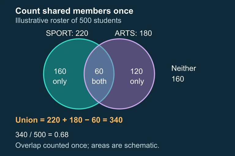 The 60 students belonging to both groups are subtracted once to avoid double counting, giving 340 of 500 in the union.
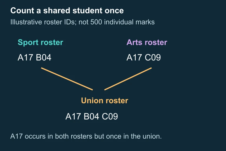 Illustrative roster showing shared ID A17 in both lists but only once in their union, alongside B04 and C09.
SECTION 7
Common Pitfalls & Misconceptions
| Misconception | Why It's Wrong | Correct Reasoning |
|---|---|---|
| "The probability of heads after five tails in a row is more than 0.5." | This is the Gambler's Fallacy. A fair coin has no memory; each flip is independent of prior outcomes. | P(Heads) = 0.5 on every flip, regardless of previous results. Independence means past outcomes do not influence future ones. |
| "Always add probabilities to find P(A or B)." | Simple addition works only for mutually exclusive events. For overlapping events, it double-counts the intersection. | Use the General Addition Rule: P(A ∪ B) = P(A) + P(B) − P(A ∩ B). Always check whether events can co-occur. |
| "If two outcomes aren't the same, they must have equal probability." | Equally likely outcomes require a symmetry argument (fair die, well-shuffled deck). Without it, outcomes may have very different probabilities. | State why outcomes are equally likely before applying the classical formula. For example, rolling a sum of 2 vs. 7 on two dice are not equally likely. |
| "A probability of 0.001 means the event will never happen." | Low probability does not mean impossible. With enough trials, even rare events occur—this is the basis of quality control and risk management. | P(A) = 0 means impossible; anything above 0 can occur. With 10,000 trials, an event with P = 0.001 is expected to occur about 10 times. |
Common probability misconceptions and corrections
KEY TAKEAWAY
SECTION 8
Connection to Conditional Probability & Independence
The probability rules introduced in this lesson form the foundation for two critical extensions: conditional probability and independence. While this lesson focuses on the unconditional probability of events, subsequent lessons explore how the probability of one event changes when we know another event has occurred. These extensions are essential for understanding Bayes' theorem, the multiplication rule for dependent events, and the design of simulation studies.
| Concept | This Lesson (Basics) | Next Steps (Advanced) |
|---|---|---|
| Event probability | P(A) computed from sample space or relative frequency | P(A | B) — probability of A given B has occurred |
| Combining events | General Addition Rule for P(A ∪ B) | General Multiplication Rule: P(A ∩ B) = P(A) × P(B | A) |
| Independence | Informal understanding; introduced but not deeply applied | Formal test: P(A ∩ B) = P(A) × P(B) iff A and B are independent |
| Applications | Describing uncertainty in single experiments | Random variables, expected value, probability distributions, and statistical inference |
How this lesson's concepts connect to advanced probability topics
Looking ahead, the probability rules from this lesson will be applied repeatedly when you study random variables (assigning numerical values to outcomes), probability distributions (the complete mapping from outcomes to probabilities), and the sampling distributions that underpin confidence intervals and significance tests. Mastering these foundational rules now ensures that the transition to inference feels like a natural extension rather than a conceptual leap.
SECTION 9
Practice Problems
Question 1: CONCEPTUAL
- A. 0.15
- B. 0.65
- C. 0.80
- D. 0.20
- E. 1.00
Show answer (C)
Question 2: BASIC CALCULATION
- A. 0.25
- B. 0.35
- C. 0.40
- D. 0.60
- E. 0.65
Show answer (D)
Question 3: INTERMEDIATE
- A. 5/6
- B. 1/6
- C. 1
- D. 13/30
- E. 30/30
Show answer (A)
Question 4: APPLIED
4 ptsShow answer
Question 5: CRITICAL THINKING
4 ptsShow answer
SUMMARY
Lesson Summary
Summary
Probability assigns a number between 0 and 1 to every event in a sample space, governed by Kolmogorov's three axioms: non-negativity, normalization (P(S) = 1), and additivity for mutually exclusive events. From these axioms follow the complement rule P(Aᶜ) = 1 − P(A) and the General Addition Rule P(A ∪ B) = P(A) + P(B) − P(A ∩ B), which corrects for double-counting when events overlap.
Probability can be interpreted through the classical (equally likely outcomes), empirical (long-run relative frequency), or subjective (personal degree of belief) lens, with the Law of Large Numbers guaranteeing that empirical frequencies converge to true probabilities. These foundational rules set the stage for conditional probability, independence, random variables, and the probability distributions that drive all of statistical inference.