Introducing Statistics: Random and Non-Random Patterns - AP Statistics

SECTION 1

Historical Context & Motivation

The question of whether an observed pattern is genuine or merely a product of chance is among the oldest intellectual puzzles in quantitative reasoning. Long before modern statistics existed as a formal discipline, gamblers, astronomers, and natural philosophers grappled with the distinction between random variation and systematic patterns. Early astronomers recording the positions of celestial bodies noticed that measurement errors seemed to scatter unpredictably around a central value, while the underlying planetary motion followed deterministic laws. This observation — that data can simultaneously contain predictable structure and unpredictable noise — became the conceptual foundation on which probability theory and statistical inference were eventually built.

1654 • Pascal-Fermat Correspondence

Blaise Pascal and Pierre de Fermat exchanged letters on the 'problem of points,' establishing the mathematical framework for reasoning about chance events and laying the groundwork for probability theory.

1733 • De Moivre's Normal Approximation

Abraham de Moivre discovered that the distribution of outcomes from repeated coin flips approaches a bell-shaped curve, providing the first mathematical characterization of how random variation behaves in aggregate.

1809 • Gauss and the Method of Least Squares

Carl Friedrich Gauss published his method of least squares for astronomical data, formally separating the systematic signal (planetary orbits) from random measurement error — a paradigm that persists in modern regression analysis.

1900 • Pearson's Chi-Square Test

Karl Pearson introduced the chi-square goodness-of-fit test, giving statisticians a formal tool to determine whether an observed distribution of data deviates from what randomness alone would predict.

1925 • Fisher's Statistical Methods

Ronald Fisher published 'Statistical Methods for Research Workers,' codifying hypothesis testing and the p-value as standard tools for distinguishing real effects from random noise in experimental data.

The central question that unites these historical developments remains at the heart of AP Statistics today: given a set of observed data, how do we determine whether the patterns we see reflect a genuine underlying structure, or whether they could plausibly have arisen from random chance alone? Answering this question requires us to first understand what randomness actually looks like, what properties it possesses, and how it differs from the deterministic or systematic patterns we seek to identify.

SECTION 2

Core Principles & Definitions

Before we can assess whether data exhibit randomness or systematic structure, we need precise definitions. In statistics, randomness does not mean chaotic or unpredictable in the colloquial sense — it means that individual outcomes are uncertain, but the long-run distribution of outcomes is governed by a stable, describable probability model. A non-random pattern, by contrast, is a systematic departure from what that probability model would predict, suggesting the presence of an explanatory factor beyond chance. The interplay between these two concepts forms the backbone of statistical reasoning, from exploratory data analysis through formal inference.

Random Process

A phenomenon whose individual outcomes cannot be predicted with certainty, but whose long-run behavior follows a known probability distribution. Examples include coin flips, random sampling, and radioactive decay.

Random Variation (Noise)

The natural, expected fluctuations in data that arise from a random process. Random variation is inherent in any dataset and does not indicate an underlying cause — it is the baseline against which we measure departures.

Systematic Pattern (Signal)

A consistent, repeatable structure in data attributable to a non-random cause. Trends, cycles, clusters, and group differences are all examples of systematic patterns that warrant explanation.

Statistical Significance

A formal determination that an observed pattern is unlikely to have arisen from random variation alone. It is typically assessed by computing the probability (p-value) of observing data as extreme as ours under a null model of pure randomness.

Probability Distribution

A mathematical function that assigns probabilities to all possible outcomes of a random variable. It serves as the model of 'what randomness looks like' against which we compare our observed data.

✦

KEY TAKEAWAY

Think of statistics as a signal-processing problem. Every dataset is like a radio broadcast: it contains the signal (the systematic pattern you want to detect) mixed with static (random noise). The statistician's job is to build a model of what pure static looks like — a probability distribution — and then determine whether the actual broadcast contains something more than static. If the observed data deviate from the static model in a way that would be very rare under chance alone, we conclude that a real signal is present.

SECTION 3

Visualizing Random vs. Non-Random Patterns

One of the most powerful ways to distinguish random from non-random behavior is to visualize data. The following diagram contrasts two sequences of observations: one generated by a truly random process, and one that contains a systematic trend embedded within random noise. Recognizing these visual signatures is an essential skill for interpreting residual plots, time-series graphs, and sampling distributions throughout the AP Statistics curriculum.

Panel A shows data generated by a random process: points scatter above and below the mean with no discernible direction or structure. Panel B shows data containing a systematic upward trend overlaid with random noise — the points still vary, but they consistently drift upward over time. Distinguishing these two patterns is the central task of statistical inference.

In Panel A, the data exhibit the hallmarks of pure random variation: there is no upward or downward drift, no clustering, and no cyclic behavior. Points fall above and below the mean with roughly equal frequency and no discernible order. In Panel B, by contrast, there is a clear systematic upward trend — even though individual observations still fluctuate around the trend line due to random noise. Recognizing this distinction visually is the first step toward understanding why formal statistical tools like hypothesis tests and confidence intervals exist: they provide a rigorous, quantitative way to decide whether a pattern like the one in Panel B is real, or whether it could plausibly have occurred by chance as in Panel A.

SECTION 4

Mathematical Framework

To formalize the distinction between random and non-random patterns, we need the language of random variables and probability distributions. A random variable is a numerical quantity whose value is determined by a random process; its probability distribution describes the relative likelihood of every possible outcome. The expected value (mean) of a random variable tells us where the center of the distribution lies, while its variance quantifies the spread of random variation around that center. Together, these two parameters establish a baseline model of 'what randomness looks like,' against which we can measure any observed departure.

EXPECTED VALUE (DISCRETE)

E(X) = μ = Σ xᵢ · P(xᵢ)

Where X is a discrete random variable, xᵢ represents each possible outcome, and P(xᵢ) is the probability of that outcome. The expected value μ is the long-run average of the random process.

VARIANCE

Var(X) = σ² = Σ (xᵢ − μ)² · P(xᵢ)

The variance σ² measures the average squared deviation of each outcome from the mean. A larger variance indicates greater random spread. The standard deviation σ = √(σ²) is the square root of variance and is expressed in the same units as X.

OBSERVED DATA MODEL

Observed Value = Systematic Component + Random Component

This is the fundamental decomposition of any observation. In regression, for instance, yᵢ = β₀ + β₁xᵢ + εᵢ, where β₀ + β₁xᵢ is the systematic part (the trend) and εᵢ is the random error term. If there is no systematic component, the observation is purely random noise centered at the mean.

The decomposition Observed = Systematic + Random is the conceptual engine of AP Statistics. When we perform a hypothesis test, our null hypothesis typically asserts that the systematic component is zero — that everything we observe is just random variation. We then ask: if the null hypothesis were true, how likely would it be to observe data as extreme as what we actually collected? If the answer is 'very unlikely,' we conclude that a non-random pattern exists. This framework applies whether we are testing a difference in means, a correlation, a proportion, or any other statistical quantity.

LAW OF LARGE NUMBERS

x̄ₙ → μ as n → ∞

As the sample size n grows, the sample mean x̄ₙ converges to the true population mean μ. This law guarantees that random variation averages out in the long run, which is why larger samples provide more reliable estimates and make it easier to detect non-random patterns.

SECTION 5

Classifying Patterns in Data

In practice, data patterns fall into several recognizable categories, and a trained statistician must be able to identify each type. Random scatter is the absence of any discernible pattern: points are distributed without trend, without clustering, and without periodicity. Trends are systematic increases or decreases over time or across an ordered variable. Clusters are groups of data points that are more similar to each other than to the rest of the data, suggesting the presence of subpopulations. Cycles are repeating patterns that occur at regular intervals, often reflecting seasonal or periodic phenomena. Each of these pattern types represents a potential non-random structure that demands investigation and explanation.

The four panels illustrate the major pattern types encountered in data analysis. Random scatter (top left) shows no structure. A linear trend (top right), clusters (bottom left), and cyclical oscillation (bottom right) all represent departures from randomness that warrant investigation.

Pattern Type	Visual Signature	Statistical Implication	Example in AP Stats
Random Scatter	No trend, no clusters, no periodicity	Consistent with null hypothesis; no evidence of systematic effect	Residual plot after a good regression fit
Linear Trend	Consistent upward or downward direction	Suggests a linear relationship between variables; non-zero slope	Scatterplot of study hours vs. exam score
Clusters	Distinct groupings separated by gaps	Suggests hidden subpopulations or confounding variables	Bimodal histogram suggesting two groups in data
Cyclical	Repeating wave-like oscillation	Suggests periodic process; may violate independence assumption	Seasonal sales data in a time-series plot

Summary of common data pattern types, their visual signatures, and AP Statistics applications

SECTION 6

Worked Example: Detecting a Non-Random Pattern

A quality control engineer at a bottling plant measures the fill volume (in ounces) of 10 consecutive bottles from the production line. The target fill is 12.00 oz. The measured values are: 12.03, 12.05, 12.07, 12.04, 12.08, 12.10, 12.09, 12.12, 12.11, 12.14. She wants to determine whether these data suggest a random process centered at 12.00 oz, or whether there is a non-random upward trend indicating that the machine is drifting out of calibration.

Analyzing Bottle Fill Data for Non-Random Patterns

1
Step 1 — Compute the Sample Mean

We first calculate the sample mean to see where the data are centered. x̄ = (12.03 + 12.05 + 12.07 + 12.04 + 12.08 + 12.10 + 12.09 + 12.12 + 12.11 + 12.14) ÷ 10 = 120.83 ÷ 10.

x̄ = 12.083 oz
2
Step 2 — Examine the Deviations from Target

All ten observations exceed 12.00 oz, with deviations +0.03,+0.05,+0.07,+0.04,+0.08,+0.10,+0.09,+0.12,+0.11,+0.14. If the deviations are independent and P(fill > 12.00) = 1/2, the probability that all ten are positive is (1/2)¹⁰ = 1/1024 ≈ 0.000977. A mean of 12.00 by itself does not imply equal probabilities above and below the target.

Under independent fair-sign assumptions: P(all ten above) = 1/1024.
3
Step 3 — Check for Trend

In order, the readings generally rise from 12.03 to 12.14 oz, with local dips. This describes the observed sample; assessing how surprising its trend is requires a specified chance model. The supplemental comparison is synthetic and is not an additional observed sample.

Upward trend detected: first observation = 12.03, last observation = 12.14 (increase of 0.11 oz)
4
Step 4 — Interpret the Results

All ten readings are above target, the sample mean is 12.083 oz, and the sequence generally rises. These observations warrant investigating the process and checking a justified chance model. Under the independent fair-sign model, ten positive deviations are unlikely, but this sample alone does not identify the cause or establish that immediate recalibration is the appropriate intervention.

Observed upward pattern: investigate the process and model assumptions before diagnosing a cause.

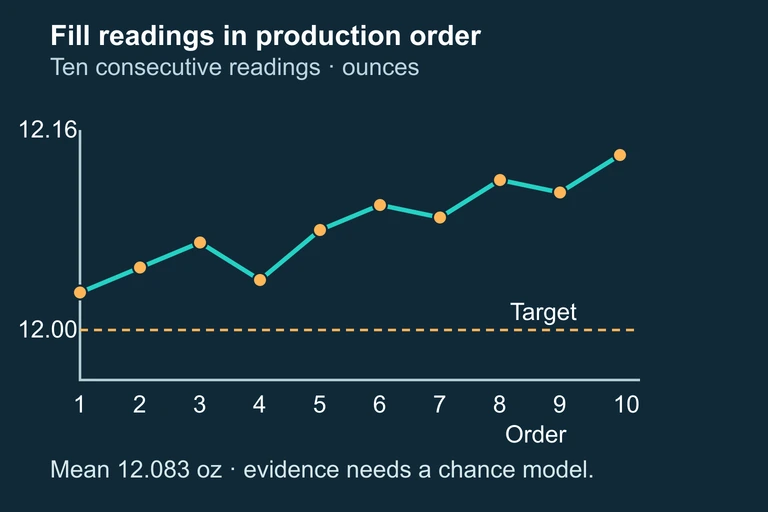Ten ordered bottle fills are above target 12.00 oz, with local dips in an overall rise. Their mean is 12.083 oz. The fill readings remain in production order; apparent trends can arise by chance, and the stated sign probability requires independent fair signs.

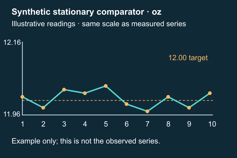Synthetic comparison fill sequence shown on the same 11.96 to 12.16 oz scale as the observed sequence.

SECTION 7

Strengths & Common Pitfalls

Distinguishing random from non-random patterns is a powerful skill, but it also comes with important caveats. Overconfidence in detecting patterns — or failure to recognize genuine randomness — can lead to flawed conclusions. The table below contrasts the strengths of pattern-recognition thinking with the most common pitfalls students encounter on the AP Statistics exam.

Strengths	Common Pitfalls
Provides a structured framework for deciding whether observed data are consistent with chance	Apophenia: seeing patterns in genuinely random data (e.g., 'hot hand' in sports, streaks in coin flips)
Applicable to any type of data — numerical, categorical, time-series, or spatial	Confusing correlation with causation: a non-random association does not prove a causal mechanism
Connects naturally to formal tools: hypothesis tests, confidence intervals, and regression	Ignoring sample size: small samples can show dramatic-looking patterns purely by chance; large samples can flag trivially small effects as 'significant'
Visual tools (scatterplots, residual plots, histograms) make pattern detection intuitive and accessible	Expecting randomness to 'look random': truly random sequences often contain streaks and clusters that look suspicious but are perfectly normal
Encourages critical thinking about data collection methods and potential biases	Multiple testing: looking at many variables increases the chance of finding a spurious 'pattern' just by luck

Comparing the analytical strengths of random vs. non-random pattern detection with the most common reasoning errors

✦

KEY TAKEAWAY

Human cognition is wired to find patterns — even where none exist. This is why statistics demands formal, probability-based criteria rather than gut feelings. Think of it like a metal detector at the beach: your eyes might see a glint in the sand and get excited, but only the detector can tell you whether it is actually metal or just a piece of mica. In the same way, hypothesis testing provides an objective 'detector' that separates real patterns from statistical mirages.

SECTION 8

Connecting to Probability Distributions & Inference

The concepts of random and non-random patterns introduced in this lesson serve as the foundation for the major probability distributions and inferential procedures you will encounter throughout AP Statistics. Understanding how randomness behaves — and what constitutes a departure from it — is precisely what enables you to construct and interpret confidence intervals, perform hypothesis tests, and evaluate regression models. The table below maps the core ideas from this lesson to their more advanced counterparts.

Concept from This Lesson	Advanced Application in AP Statistics
Random variation around a mean	Normal distribution: models how random measurements cluster around μ with spread σ; basis for z-tests and t-tests
Probability of observing outcomes by chance	Binomial and geometric distributions: count successes or trials in a random process with fixed probability p
Decomposition: Observed = Systematic + Random	Linear regression: yᵢ = β₀ + β₁xᵢ + εᵢ; residuals εᵢ should show random scatter if model is correct
Identifying non-random trends in data	Hypothesis testing: H₀ asserts 'randomness only'; if data are extreme under H₀, we reject in favor of Hₐ
Law of Large Numbers (sample mean → μ)	Sampling distributions and the Central Limit Theorem: the distribution of x̄ becomes approximately normal as n increases

Mapping introductory concepts to their advanced counterparts in the AP Statistics curriculum

As you progress through the course, every new topic will fundamentally rely on the question posed in this lesson: Is the pattern I observe random or non-random? When you construct a confidence interval, you are quantifying the range of values consistent with random variation around an estimated parameter. When you perform a chi-square test, you are measuring how far observed category counts deviate from what randomness predicts. When you examine a residual plot, you are checking whether the leftovers from your model look like random noise. Mastering the intuition for random versus non-random patterns now will pay dividends in every subsequent unit of the course.

SECTION 9

Practice Problems

Question 1: CONCEPTUAL

A researcher flips a fair coin 100 times and observes 58 heads. She notes that this is more than the expected 50 heads and concludes the coin must be biased. Which of the following best explains the flaw in her reasoning?

A. A fair coin should always produce exactly 50 heads in 100 flips.
B. Random variation means that outcomes from a fair coin will naturally fluctuate around the expected value, so 58 heads out of 100 is within the range of plausible outcomes for a fair coin.
C. She should have flipped the coin exactly 1,000 times before drawing any conclusions.
D. The Law of Large Numbers guarantees that the proportion of heads will equal exactly 0.50 in any sufficiently large sample.
E. 58 heads is statistically impossible for a fair coin.

Show answer (B)

Correct Answer: B. Random variation is an inherent feature of any random process, meaning that the observed proportion of heads will naturally fluctuate around 0.50 from sample to sample. For 100 flips of a fair coin, the standard deviation of the number of heads is √(100 × 0.5 × 0.5) = 5, so 58 heads is only 1.6 standard deviations above the mean — well within the range of typical random fluctuation. Choice A is wrong because a fair coin is not expected to produce exactly 50 heads — it is expected to produce 50 on average, with variation around that value. Choice C is wrong because while larger samples improve precision, no specific sample size is required before one can reason about data. Choice D mischaracterizes the Law of Large Numbers, which guarantees convergence in the limit, not exact equality at any finite sample size. Choice E is wrong because 58 heads is entirely possible for a fair coin.

Question 2: BASIC CALCULATION

A random variable X has the following probability distribution: P(X = 1) = 0.2, P(X = 2) = 0.3, P(X = 3) = 0.3, P(X = 4) = 0.2. What is the expected value E(X) and the variance Var(X)?

A. E(X) = 2.5, Var(X) = 1.05
B. E(X) = 2.5, Var(X) = 1.00
C. E(X) = 2.5, Var(X) = 1.25
D. E(X) = 2.5, Var(X) = 1.10
E. E(X) = 2.0, Var(X) = 1.10

Show answer (A)

Correct Answer: A. Compute the expected value: E(X) = 1(0.2) + 2(0.3) + 3(0.3) + 4(0.2) = 0.2 + 0.6 + 0.9 + 0.8 = 2.5. Compute E(X²): E(X²) = 1²(0.2) + 2²(0.3) + 3²(0.3) + 4²(0.2) = 0.2 + 1.2 + 2.7 + 3.2 = 7.3. Apply the variance formula: Var(X) = E(X²) − [E(X)]² = 7.3 − (2.5)² = 7.3 − 6.25 = 1.05. This result can be confirmed using the definition directly: Var(X) = (1 − 2.5)²(0.2) + (2 − 2.5)²(0.3) + (3 − 2.5)²(0.3) + (4 − 2.5)²(0.2) = (2.25)(0.2) + (0.25)(0.3) + (0.25)(0.3) + (2.25)(0.2) = 0.45 + 0.075 + 0.075 + 0.45 = 1.05. Choice A is correct: E(X) = 2.5 and Var(X) = 1.05. Choice B is wrong because Var(X) ≠ 1.00. Choice C is wrong because Var(X) ≠ 1.25. Choice D is wrong because Var(X) ≠ 1.10. Choice E is wrong because E(X) ≠ 2.0.

Question 3: INTERMEDIATE

A student fits a least-squares regression line to a scatterplot of temperature (x) versus ice cream sales (y). The residual plot shows a clear U-shaped (curved) pattern. Which of the following is the most appropriate interpretation?

A. The linear model is appropriate because all residuals are close to zero.
B. The residuals exhibit a non-random pattern, indicating that the linear model does not adequately capture the relationship; a nonlinear model may be more appropriate.
C. The U-shaped pattern confirms that ice cream sales cause higher temperatures.
D. The curved residual pattern is a consequence of random variation and should be ignored.
E. The regression line should be recalculated after removing the outliers that create the U-shape.

Show answer (B)

Correct Answer: B. A residual plot should show random scatter if the model fits well. A U-shaped (curved) pattern is a classic non-random structure indicating that the linear model fails to capture the true relationship between the variables. This systematic pattern in the residuals means a nonlinear model (such as a quadratic or logarithmic transformation) would likely provide a better fit. Choice A is wrong because the presence of a U-shape means residuals are systematically positive at low and high x-values and negative in the middle — this is not 'close to zero' in a random sense. Choice C incorrectly infers causation from an association. Choice D dismisses a clear systematic pattern as random noise, which contradicts the core principle of residual analysis. Choice E incorrectly assumes the pattern is caused by outliers; a U-shape across the full range of data is a model specification issue, not an outlier issue.

Question 4: APPLIED

4 pts

A hospital administrator collects the number of emergency room visits per day for 14 consecutive days. The data are: 42, 45, 44, 48, 50, 47, 52, 55, 53, 58, 56, 60, 59, 63. (a) Calculate the sample mean and describe the overall pattern you observe in the data. (b) Describe one specific non-random feature of this dataset and explain why it suggests the data are not generated by a stable random process. (c) Suppose someone claims the data are randomly fluctuating around a constant mean. Explain why this claim is not well-supported by the evidence. (d) Suggest one real-world factor that could explain the non-random pattern and describe how you might investigate it.

Show answer

Rubric (4 points): Part (a) — 1 point: The sample mean is x̄ = (42 + 45 + 44 + 48 + 50 + 47 + 52 + 55 + 53 + 58 + 56 + 60 + 59 + 63) ÷ 14 = 732 ÷ 14 = 52.29 visits per day (approximately). The overall pattern shows a general increase in ER visits over the 14-day period, from 42 at the start to 63 at the end. Award 1 point for correct calculation of the mean AND a description that the data generally increase over time. Part (b) — 1 point: A specific non-random feature is the upward trend: the first seven values range from 42–52, while the last seven range from 53–63. This consistent shift upward would be very unlikely if the data were randomly varying around a fixed mean, because we would expect values to be roughly evenly distributed above and below the mean throughout the sequence. Award 1 point for identifying a specific non-random feature (trend, runs, or increasing mean) AND explaining why it contradicts randomness. Part (c) — 1 point: If the data were randomly fluctuating around a constant mean, we would expect approximately equal numbers of values above and below that mean scattered throughout the time period, with no directional drift. Instead, the early observations are almost all below the overall mean (52.29) and the late observations are almost all above it. This systematic time-ordering of residuals is inconsistent with random variation. Award 1 point for a clear explanation referencing the expected behavior under randomness AND contrasting it with the observed behavior. Part (d) — 1 point: A plausible real-world factor could be the onset of flu season, an emerging disease outbreak, or a community event increasing injury rates. To investigate, the administrator could extend the data collection over several more weeks to confirm the trend continues, compare ER diagnoses across the time period to identify whether a particular type of visit is driving the increase, or examine whether similar trends occurred in previous years. Award 1 point for identifying a plausible real-world cause AND proposing a reasonable investigative strategy.

Question 5: CRITICAL THINKING

4 pts

A statistics student simulates 200 rolls of a fair six-sided die on a computer. She then examines the entire sequence and notices that the number 4 appears five times in a row between rolls 87 and 91. She concludes that the random number generator must be broken because "true randomness wouldn't produce such a streak." (a) Calculate the probability of rolling five consecutive 4s in a specific, predetermined set of five rolls of a fair six-sided die. Show your work. (b) Explain why observing a streak of five identical values somewhere in a sequence of 200 rolls is much more likely than the probability you calculated in part (a). Include a numerical estimate to support your explanation. (c) Discuss the general principle about the difference between the probability of a specific rare event at a predetermined location versus the probability of finding that rare event somewhere in a large dataset. How does this connect to the student's error in reasoning? (d) How does this scenario illustrate the concept that humans often misjudge what randomness looks like? Why does this matter for statistical practice?

Show answer

Rubric (4 points): Part (a) — 1 point: The probability of rolling a 4 on any single roll of a fair six-sided die is 1/6. Because the rolls are independent, the probability of rolling five consecutive 4s in five specific, predetermined rolls is: P = (1/6)⁵ = 1/7776 ≈ 0.000129, or approximately 0.013%. Award 1 point for a correct calculation showing (1/6)⁵ = 1/7776 with a correct numerical approximation. Part (b) — 1 point: In a sequence of 200 rolls, there are 196 possible starting positions where a run of 5 consecutive identical values could begin (positions 1 through 196). Furthermore, the streak does not have to consist of 4s specifically — a run of five consecutive 1s, 2s, 3s, 5s, or 6s would be equally notable. Using a simplified approximation, the expected number of such runs is roughly 196 × 6 × (1/6)⁵ = 196 × (1/1296) ≈ 0.151, meaning there is roughly a 14–15% chance of observing at least one such streak somewhere in the sequence (using 1 −

e^{−0.151}

≈ 0.14 as a Poisson approximation). This is far higher than 0.013% because the large number of opportunities for a streak multiplies the overall likelihood. Note: The factor of 6 accounts for the fact that any of the six face values could form the streak, and the 196 accounts for the many possible starting positions. The approximation ignores overlap between windows but captures the key insight. Award 1 point for explaining that there are many possible locations in the sequence where a streak could occur and that the streak could involve any face value, which substantially increases the overall probability compared to a single predetermined location and value. Part (c) — 1 point: This scenario illustrates the distinction between pre-specified and post-hoc (after-the-fact) probabilities. The probability of a specific rare event occurring at a specific predetermined position is very low. However, the probability that some rare-looking event occurs somewhere in a large dataset is much higher, because the large number of opportunities provides many chances for the event to happen. This principle is closely related to the multiple comparisons or multiple testing problem: when we search through large amounts of data looking for patterns after the fact, we will almost inevitably find something that looks surprising, even if the data are entirely random. The student made the error of calculating (or intuiting) the probability for a specific location and specific value and then applying that tiny probability as if it described the chance of seeing any such streak anywhere in the full sequence. Award 1 point for clearly articulating the general principle that the probability of finding a rare pattern anywhere in a large dataset is much higher than the probability of finding one at a specific predetermined location, and for connecting this to the idea that searching after the fact inflates the apparent significance of discovered patterns. Part (d) — 1 point: Humans tend to expect random sequences to look more evenly spread out than they actually are. Psychological research shows that people systematically underestimate the frequency of streaks, clusters, and runs in truly random data. The student's reaction — concluding that the random number generator must be broken — reflects this well-documented cognitive bias known as the representativeness heuristic: people expect each short segment of a random sequence to mirror the overall long-run proportions, so any local clustering feels non-random. In reality, true randomness routinely produces local patterns that appear non-random to the human eye. This scenario demonstrates precisely why formal statistical tools — rather than visual intuition alone — are necessary for rigorously distinguishing genuine non-random patterns from artifacts of chance. A proper statistical test would compare the observed frequency and length of streaks to what is expected under randomness before drawing any conclusions about whether the generator is flawed. Award 1 point for discussing the human tendency to misjudge what randomness looks like (e.g., expecting too much alternation and too few streaks) and connecting it to the need for formal statistical methods rather than informal visual inspection.

SUMMARY

Lesson Summary

Summary

This lesson introduced the fundamental distinction at the heart of AP Statistics: the difference between random variation (the natural, expected fluctuations produced by chance processes) and non-random patterns (systematic structures in data that suggest a cause beyond chance). We formalized this through the decomposition Observed = Systematic + Random, and we introduced the expected value and variance as the two parameters that characterize a probability distribution — the mathematical model of what randomness looks like.

We identified four key pattern types — random scatter, trends, clusters, and cycles — and learned that only random scatter is consistent with pure chance. We explored common pitfalls, including apophenia (seeing patterns in noise) and the multiple testing problem, and connected this lesson's concepts to the full arc of AP Statistics: normal distributions, hypothesis testing, regression, and the Central Limit Theorem. The ability to distinguish signal from noise is the single most important skill you will develop in this course.