Introducing Statistics: Are My Results Unexpected? - AP Statistics

SECTION 1

Historical Context & Motivation

Statistics has always been driven by a fundamental question: Could this result have happened by chance alone? In the late nineteenth and early twentieth centuries, scientists working with categorical data—counts of organisms, disease outcomes, genetic phenotypes—needed a formal method to decide whether observed frequencies deviated meaningfully from theoretical expectations. The development of the chi-square (χ²) test gave researchers exactly that tool, transforming intuitive suspicion into rigorous inference.

1857 • Gregor Mendel's Pea Experiments

Mendel compared observed ratios of pea phenotypes (smooth vs. wrinkled, yellow vs. green) against predicted 3:1 ratios, performing informal goodness-of-fit reasoning decades before a formal test existed.

1900 • Karl Pearson Proposes χ²

Karl Pearson published 'On the Criterion that a Given System of Deviations from the Probable in the Case of a Correlated System of Variables is Such that it Can Be Reasonably Supposed to Have Arisen from Random Sampling,' introducing the chi-square goodness-of-fit statistic.

1922 • Ronald Fisher Refines Degrees of Freedom

Fisher corrected Pearson's original degrees-of-freedom calculation and extended the chi-square framework, clarifying how to account for estimated parameters and paving the way for tests of independence and homogeneity.

1952 • Widespread Adoption in Social Sciences

By mid-century, chi-square tests had become standard practice in genetics, psychology, political science, and public health, enabling researchers to evaluate categorical outcomes in survey data and experimental studies alike.

The central gap these pioneers addressed is one you will encounter constantly on the AP Statistics exam and in research: when your observed data differ from the counts you expected under some hypothesis, how do you determine whether the discrepancy is just sampling variability or evidence that the hypothesis is wrong? The chi-square statistic provides a single number that quantifies the total discrepancy, and the chi-square distribution tells you how likely that discrepancy is if the hypothesis were true.

SECTION 2

Core Principles & Definitions

Before computing anything, you need to understand the foundational concepts that underpin all chi-square inference. These ideas connect the raw counts you collect to the probabilistic reasoning that drives your conclusion. Whether you are testing whether a die is fair, whether two categorical variables are associated, or whether several populations share the same distribution of responses, the same core logic applies.

Observed Counts (O)

The actual frequencies you record from your sample. Each observation falls into exactly one category, and you tally the totals. These are the raw data that drive every chi-square calculation.

Expected Counts (E)

The frequencies you would predict if the null hypothesis were true. Expected counts are computed from the hypothesized model—proportions, row and column totals, or a specific distribution—and must always be calculated, never observed.

Chi-Square Statistic (χ²)

A single non-negative number that aggregates the squared, standardized deviations between observed and expected counts across all categories. Larger values indicate greater discrepancy from the null hypothesis.

Degrees of Freedom (df)

The number of independent pieces of information in your data table once constraints (like fixed totals) are imposed. For a goodness-of-fit test with k categories, df = k − 1. Degrees of freedom determine which chi-square distribution to reference.

P-Value

The probability of obtaining a χ² statistic at least as large as yours, assuming the null hypothesis is true. A small p-value (typically below α = 0.05) provides convincing evidence against the null.

✦

KEY TAKEAWAY

Think of expected counts as the blueprint for a building and observed counts as the building you actually constructed. The chi-square statistic measures the total amount of deviation between your blueprint and the finished structure. Small deviations happen naturally (lumber varies slightly, walls shift a millimeter), but if the front door ends up on the second floor, you have strong evidence the builders weren't following the blueprint. Similarly, a large χ² tells you the data likely did not arise from the hypothesized model.

SECTION 3

Visualizing Observed vs. Expected

The best way to build intuition about chi-square inference is to see the gap between what you expected and what you observed. The diagram below illustrates a simple scenario: you roll a six-sided die 120 times and record the frequency for each face. Under the null hypothesis that the die is fair, you expect each face to appear 20 times. The cyan bars represent observed counts, the dashed line marks the expected count, and the shaded regions highlight the deviations that the chi-square statistic will quantify.

Each cyan bar represents the observed frequency for a die face. The amber dashed line at 20 marks the expected count under the fair-die hypothesis. Red-shaded regions highlight the magnitude of each deviation. Face 4 shows the largest positive deviation (+10), while face 6 shows the largest negative deviation (−8).

Notice that looking at individual deviations alone does not give you the complete picture. Face 3 matches the expectation perfectly, while faces 4 and 6 diverge substantially in opposite directions. The chi-square statistic will combine all of these deviations into a single summary measure that accounts for both the size of each deviation and the expected count against which it is measured. This aggregation is what allows you to make a single inferential decision rather than evaluating six separate deviations one by one.

SECTION 4

Mathematical Framework

The mathematical backbone of chi-square inference is elegantly simple: you measure how far each observed count is from its expected value, square the difference to eliminate signs, divide by the expected count to standardize, and sum across all categories. The resulting statistic follows, approximately, a chi-square distribution whose shape depends on the degrees of freedom.

CHI-SQUARE TEST STATISTIC

χ² = Σ (O − E)² / E

where O = observed count in a category, E = expected count in that same category, and the sum is taken over all k categories.

Each term in the sum, (O − E)² / E, is the contribution from one cell or category. Squaring the numerator ensures that positive and negative deviations both increase χ². Dividing by E standardizes the contribution: a deviation of 5 when the expected count is 10 is proportionally much more surprising than the same deviation of 5 when the expected count is 500. This standardization is critical because it places every category on a comparable scale.

DEGREES OF FREEDOM — GOODNESS-OF-FIT

df = k − 1

where k = the number of categories. One degree of freedom is lost because the category counts must sum to the fixed total n.

EXPECTED COUNT — GOODNESS-OF-FIT

E = n × p₀

where n = total sample size and p₀ = the hypothesized proportion for that category. For a test of independence in a two-way table, E = (row total × column total) / n.

⚠

Conditions for Inference

Before performing a chi-square test, three conditions must be verified: (1) the data come from a random sample or random assignment, (2) the sample is independent (if sampling without replacement, n ≤ 10% of the population), and (3) all expected counts are at least 5 so the chi-square approximation is reliable. If any expected count falls below 5, consider combining categories or using an alternative exact test.

SECTION 5

The Chi-Square Distribution & P-Values

Once you compute the χ² statistic, you need a reference distribution to determine how extreme that value is. The chi-square distribution is a family of right-skewed distributions parameterized by degrees of freedom. As df increases, the distribution becomes more symmetric and shifts to the right. The p-value is always calculated as the area in the right tail because larger χ² values represent greater discrepancies from the null hypothesis. Unlike a t-test, there is no two-sided or left-tail version: chi-square tests are inherently one-directional in the sense that only large values of χ² provide evidence against H₀.

Three chi-square density curves for df = 3 (cyan), df = 5 (violet), and df = 10 (amber). All are right-skewed and non-negative. As degrees of freedom increase, the center of the distribution shifts right and the shape becomes less skewed. The shaded violet region illustrates the p-value: the area under the df = 5 curve to the right of a particular χ² value.

On the AP exam, you will typically use your calculator's χ²cdf function or a chi-square table to find the p-value. On the TI-83/84, the command is χ²cdf(χ²stat, 1E99, df), which returns the probability in the right tail from your test statistic to positive infinity. The key interpretive point is straightforward: if the p-value is less than your significance level α, you reject H₀ and conclude that the observed distribution of counts is significantly different from what the null hypothesis predicted.

SECTION 6

Worked Example: Is This Die Fair?

Let us return to the die-rolling scenario from Section 3. You suspect a six-sided die may be loaded, so you roll it 120 times and record the following frequencies: Face 1 → 25, Face 2 → 15, Face 3 → 20, Face 4 → 30, Face 5 → 18, Face 6 → 12. Perform a chi-square goodness-of-fit test at the α = 0.05 significance level.

Chi-Square Goodness-of-Fit: Fair Die

1
Step 1 — State Hypotheses

H₀: The die is fair; each face has probability p = 1/6. Hₐ: The die is not fair; at least one face has a probability different from 1/6.
2
Step 2 — Check Conditions

Assume the 120 rolls are independent (reasonable for a physical die). Each expected count is E = 120 × (1/6) = 20, which satisfies the requirement that all expected counts be at least 5. The conditions for a chi-square goodness-of-fit test are met.

All expected counts = 20 ≥ 5 ✓
3
Step 3 — Compute the Chi-Square Statistic

χ² = (25 − 20)²/20 + (15 − 20)²/20 + (20 − 20)²/20 + (30 − 20)²/20 + (18 − 20)²/20 + (12 − 20)²/20 = 25/20 + 25/20 + 0/20 + 100/20 + 4/20 + 64/20 = 1.25 + 1.25 + 0 + 5.00 + 0.20 + 3.20 = 10.90

χ² = 10.90
4
Step 4 — Determine Degrees of Freedom & P-Value

df = k − 1 = 6 − 1 = 5. Using a calculator: χ²cdf(10.90, 1E99, 5) ≈ 0.0534. Alternatively, consulting a chi-square table, the critical value for df = 5 at α = 0.05 is 11.07.

p-value ≈ 0.0534, df = 5
5
Step 5 — State the Conclusion in Context

Since the p-value (≈ 0.0534) is greater than α = 0.05, we fail to reject H₀. There is not sufficient evidence at the 5% significance level to conclude that the die is unfair. While the deviations are noticeable—particularly for faces 4 and 6—they are not statistically significant by this standard. Note, however, that the result is borderline; a researcher using α = 0.10 would reject H₀.

Fail to reject H₀ at α = 0.05. Insufficient evidence that the die is unfair.

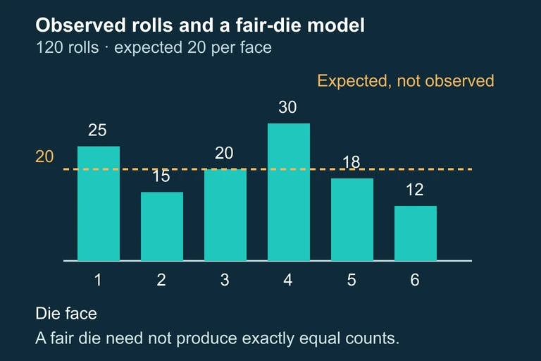Six observed die-face counts 25,15,20,30,18,12 sum to 120. The fair-model expected count is 20 per face. Observed face counts total 120, while the fair-die model expects 20 per face; one fair run need not match those expectations exactly.

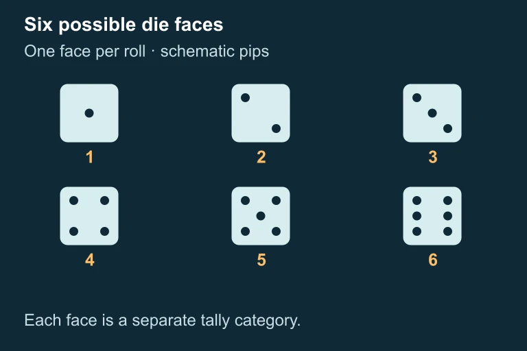Six labeled die-face icons with exactly one through six pips.

SECTION 7

Strengths, Limitations & Common Pitfalls

The chi-square test is remarkably versatile and appears throughout the AP Statistics curriculum in three forms—goodness-of-fit, test of independence, and test of homogeneity—but it is not without limitations. Understanding where the test shines and where it breaks down will help you choose the right inferential tool and avoid common exam mistakes.

Strengths	Limitations	Common Pitfalls on the AP Exam
Works with categorical (nominal or ordinal) data—no normality assumption on the variable itself.	Requires all expected counts ≥ 5; small expected counts make the chi-square approximation unreliable.	Using observed counts where expected counts belong in the denominator of the χ² formula.
Easy to compute by hand and by calculator; the formula is the same for all three chi-square tests.	Cannot indicate the direction or nature of the association—only that a discrepancy exists.	Forgetting to state hypotheses in context (e.g., writing generic H₀ instead of referencing the specific variables).
Applicable to a wide range of research designs: surveys, experiments, observational studies.	Sensitive to sample size: with very large n, even trivially small deviations become 'significant.'	Confusing the test of independence (one sample, two variables) with the test of homogeneity (multiple populations, one variable).
Only requires counts; no need to assume equal variances or specific distributional shapes.	Not appropriate for paired or matched data; observations must be independent.	Failing to check the expected count condition or the random sampling / independence condition.

Summary of strengths, limitations, and common AP exam pitfalls for chi-square tests

✦

KEY TAKEAWAY

The chi-square statistic is like a smoke detector: it tells you something is off, but not which room is on fire. A significant χ² indicates that at least one category's observed count differs meaningfully from its expected count, but to identify which categories are driving the significance, you must inspect the individual (O − E)² / E components. The largest components point to the categories with the most surprising deviations—this is your follow-up analysis.

SECTION 8

Connecting to Advanced Chi-Square Tests

The goodness-of-fit test you have just learned is the simplest member of the chi-square family. The AP Statistics exam also requires mastery of two closely related tests that use the same χ² = Σ(O − E)² / E formula but apply it to two-way tables. Understanding the relationships among these three tests—and how they differ in design and hypotheses—is essential for exam success.

Feature	Goodness-of-Fit	Test of Independence	Test of Homogeneity
Number of variables	One categorical variable	Two categorical variables	One categorical variable across multiple populations
Number of samples	One sample	One sample	Two or more independent samples
Null hypothesis	The variable follows a specified distribution	The two variables are independent (no association)	The distribution of the variable is the same across all populations
Degrees of freedom	k − 1	(r − 1)(c − 1)	(r − 1)(c − 1)
How E is computed	E = n × p₀ from hypothesized proportions	E = (row total × column total) / n	E = (row total × column total) / n

Comparison of the three chi-square tests on the AP Statistics exam

As you progress through the chi-square unit, you will see that the test of independence and the test of homogeneity are computationally identical—the same formula, the same degrees of freedom, the same expected-count calculation. The distinction is entirely about study design and interpretation. The test of independence asks whether two variables are associated within a single population, while the test of homogeneity asks whether the distribution of a single variable is the same across several populations or treatments. This distinction frequently appears in free-response questions, so practice identifying the study design before you begin computing.

SECTION 9

Practice Problems

Question 1: CONCEPTUAL

In a chi-square goodness-of-fit test, why is each (O − E) term squared before dividing by E?

A. To make the computation easier to perform by hand.
B. To prevent positive and negative deviations from canceling each other out.
C. To convert the test statistic into a z-score.
D. To ensure the chi-square statistic is always less than 1.
E. To adjust for the fact that expected counts are estimated.

Show answer (B)

Correct answer: B. Squaring each deviation (O − E) is essential because some observed counts will be above the expected value (positive deviation) while others will be below (negative deviation). Without squaring, these deviations could sum to zero even when the data depart substantially from the null hypothesis. A is incorrect because squaring does not simplify computation—it adds a step. C is incorrect because the chi-square statistic is not a z-score; it follows a chi-square distribution, not a standard normal. D is incorrect because χ² can take any non-negative value, including values much greater than 1. E is incorrect; the division by E is what standardizes for the magnitude of the expected count, not the squaring.

Question 2: BASIC CALCULATION

A genetics researcher expects offspring phenotypes in a 9:3:3:1 ratio. In a sample of 160 offspring, the observed counts are 85, 35, 26, and 14. What is the expected count for the category with the 3/16 proportion?

A. 10
B. 26
C. 30
D. 35
E. 90

Show answer (C)

Correct answer: C. The expected count is calculated as E = n × p₀ = 160 × (3/16) = 30. A (10) equals 160 × 1/16, which is the expected count for the rarest category, not the 3/16 category. B (26) is the observed count for the third category, not the expected count. D (35) is the observed count for the second category. E (90) equals 160 × 9/16, the expected count for the most common category.

Question 3: INTERMEDIATE

A marketing analyst surveys 200 randomly selected customers about their preferred product color. Under the null hypothesis that preferences are equally distributed among Red, Blue, Green, and Yellow, the observed counts are 60, 55, 45, and 40. Which of the following is closest to the chi-square test statistic?

A. 3.0
B. 4.6
C. 5.0
D. 7.8
E. 10.0

Show answer (C)

Correct answer: C. With equal distribution and n = 200 across 4 categories, E = 200/4 = 50 for each. χ² = (60 − 50)²/50 + (55 − 50)²/50 + (45 − 50)²/50 + (40 − 50)²/50 = 100/50 + 25/50 + 25/50 + 100/50 = 2.0 + 0.5 + 0.5 + 2.0 = 5.0. A (3.0) would result from underestimating the Red and Yellow contributions. B (4.6) may arise from a rounding error in an intermediate step. D (7.8) is the critical value for df = 3 at α = 0.05, not the test statistic. E (10.0) could result from forgetting to divide each squared deviation by E.

Question 4: APPLIED

4 pts

A public health researcher collects data from 500 randomly selected hospital patients to determine whether the distribution of blood types in a city matches the national distribution: Type O (44%), Type A (42%), Type B (10%), Type AB (4%). The observed counts are: O = 235, A = 195, B = 50, AB = 20. (a) State appropriate hypotheses for a chi-square goodness-of-fit test. (b) Calculate the expected counts and verify the conditions for inference. (c) Compute the chi-square test statistic. (d) Using df = 3 and the chi-square distribution, determine the p-value range and state your conclusion at α = 0.05.

Show answer

Rubric (4 points): Point 1 — Hypotheses: H₀: The distribution of blood types in the city matches the national distribution (

p_O

= 0.44,

p_A

= 0.42,

p_B

= 0.10, p_AB = 0.04). Hₐ: The distribution of blood types in the city does not match the national distribution (at least one proportion differs). Point 2 — Expected counts and conditions: E(O) = 500 × 0.44 = 220, E(A) = 500 × 0.42 = 210, E(B) = 500 × 0.10 = 50, E(AB) = 500 × 0.04 = 20. All expected counts ≥ 5 ✓. The problem states the sample is randomly selected and 500 is almost certainly less than 10% of all hospital patients (independence condition). ✓ Point 3 — Test statistic: χ² = (235 − 220)²/220 + (195 − 210)²/210 + (50 − 50)²/50 + (20 − 20)²/20 = 225/220 + 225/210 + 0/50 + 0/20 = 1.023 + 1.071 + 0 + 0 ≈ 2.094. Point 4 — P-value and conclusion: Using χ²cdf(2.094, 1E99, 3) ≈ 0.553. Since p-value ≈ 0.553 > 0.05 = α, we fail to reject H₀. There is not convincing evidence that the distribution of blood types in the city differs from the national distribution.

Question 5: CRITICAL THINKING

4 pts

A student conducts a chi-square goodness-of-fit test on whether a spinner with five equal sections lands on each section with equal probability. She spins 50 times and obtains χ² = 9.2 with df = 4 and a p-value of 0.056. She repeats the experiment with 500 spins, observing the same proportional deviations (i.e., the relative discrepancies between observed and expected are identical to the first experiment). (a) Without computing, explain whether the new χ² will be larger, smaller, or the same as 9.2, and justify your reasoning. (b) Explain the implications for the p-value and the statistical conclusion. (c) Discuss whether this means the spinner is "more unfair" in the second experiment. (d) Propose a way to communicate both statistical significance and practical significance for this scenario.

Show answer

Rubric (4 points): Point 1 — Effect of sample size on χ²: The new χ² will be larger. The chi-square statistic scales linearly with sample size when the proportional deviations remain constant. Since each (O − E)² / E term has E proportional to n, and (O − E)² is proportional to n² when the proportional deviation is fixed, each component is proportional to n. Multiplying the sample size by 10 multiplies χ² by approximately 10, giving χ² ≈ 92. Point 2 — Implications for p-value: With χ² ≈ 92 and df = 4, the p-value will be extremely small (essentially 0). The student would now reject H₀ at any conventional significance level. The borderline result (p = 0.056) became overwhelmingly significant simply because of increased sample size. Point 3 — Practical vs. statistical significance: The spinner is not "more unfair" in the second experiment—the same proportional deviations exist. The chi-square test detected the discrepancy more reliably with a larger sample. Statistical significance does not equal practical significance; a very large sample can detect trivially small departures from the null that have no real-world consequence. Point 4 — Communicating practical significance: The student could report the actual observed proportions alongside the expected proportions and compute an effect size measure such as Cramér's V or the relative deviation for each category. This allows the reader to judge whether the departure from equal probability is large enough to matter in context (e.g., for a board game, a deviation of 1–2 percentage points per section is negligible).

SUMMARY

Summary & Key Concepts

Summary

The central question in this lesson—Are my results unexpected?—is answered by computing the chi-square statistic χ² = Σ(O − E)² / E, which measures the total standardized discrepancy between observed counts and expected counts under a null hypothesis. Large values of χ² signal that the data are unlikely to have arisen from the hypothesized model, and the p-value—the right-tail area under the chi-square distribution with the appropriate degrees of freedom—quantifies how surprising the observed discrepancy is.

Before computing, always verify three conditions: the data come from a random sample or random assignment, observations are independent, and all expected counts are at least 5. The goodness-of-fit test introduced here uses df = k − 1 and compares one sample's distribution to a hypothesized model. This same logic extends to the test of independence and the test of homogeneity in two-way tables, where expected counts are calculated as (row total × column total) / n and degrees of freedom are (r − 1)(c − 1). Mastering this foundational framework prepares you for all chi-square inference on the AP exam.