Introducing Statistics: Why Is My Sample Not Like Yours? - AP Statistics

SECTION 1

Historical Context & Motivation

Statistics was born from a practical dilemma: how can we draw reliable conclusions about a large group when we can only observe a small part of it? Long before modern polling and clinical trials, scholars recognized that individual observations are inherently noisy, and that patterns become clear only when data are aggregated thoughtfully. The concept of sampling variability — the idea that different samples drawn from the same population will yield different results — is the engine that drives all of statistical inference. Understanding why your sample is not like mine is the first step toward quantifying uncertainty and making evidence-based decisions.

1713 • Bernoulli's Ars Conjectandi

Jacob Bernoulli posthumously published the first formal proof that sample proportions converge to population proportions as sample size grows — the precursor to the Law of Large Numbers.

1809 • Gauss and the Normal Curve

Carl Friedrich Gauss demonstrated that measurement errors follow a bell-shaped distribution, establishing the normal distribution as a cornerstone of probability theory.

1908 • Student's t-Distribution

William Sealy Gosset, publishing under the pseudonym "Student," derived the t-distribution to handle small-sample inference — showing that sample variability matters most when data are scarce.

1933 • Neyman's Confidence Intervals

Jerzy Neyman introduced the framework of repeated sampling to define confidence intervals, formally connecting sampling distributions to practical inference.

1948 • Modern Survey Sampling

The publication of Cochran's Sampling Techniques codified probability-based sampling designs, making rigorous inference from samples a standard practice across the sciences and social research.

The central question that links all of these developments is deceptively simple: if I draw one random sample and you draw another, why should we expect different results, and how different should we expect them to be? Answering this question requires a precise understanding of sampling distributions — the theoretical distributions that describe how a statistic behaves across all possible samples of a given size.

SECTION 2

Core Principles & Definitions

Before examining the mathematics, it is essential to anchor the vocabulary that AP Statistics expects you to command. The distinction between a parameter and a statistic underpins everything: a parameter is a fixed numerical characteristic of a population (such as the true mean μ or the true proportion p), whereas a statistic is the corresponding value calculated from a sample (such as x̄ or p̂). Because the sample is random, every statistic is a random variable, and its distribution across all possible samples of size n is the sampling distribution.

Population vs. Sample

The population is the entire group of interest; the sample is the subset actually observed. Inference flows from sample to population.

Parameter vs. Statistic

Parameters (μ, σ, p) are fixed but usually unknown. Statistics (x̄, s, p̂) are computed from data and vary from sample to sample.

Sampling Variability

Different random samples produce different statistics. This natural fluctuation is sampling variability — it is not error but an expected feature of randomness.

Sampling Distribution

The sampling distribution of a statistic is the probability distribution of that statistic over all possible samples of a fixed size n from the population.

Bias and Variability

An estimator is unbiased if the mean of its sampling distribution equals the parameter. Low variability means the estimates cluster tightly around that center.

SECTION 3

Visualizing Sampling Variability

The diagram below illustrates the core idea: a single population gives rise to many possible samples, each of which produces its own sample mean. Collecting these sample means into a histogram reveals the sampling distribution of x̄. Notice that while each individual sample mean differs, their collective distribution has a predictable center and spread.

A population with μ = 50 and σ = 10 produces many samples of size n = 25. Each sample yields a different x̄. The histogram of all possible x̄ values forms the sampling distribution, centered at μ = 50 with standard error σ/√n = 2.

Several features of this diagram deserve attention. First, the center of the sampling distribution coincides with the population mean μ — this is the defining property of an unbiased estimator. Second, the spread of the sampling distribution is considerably smaller than the population's own spread. While individual observations range widely (σ = 10), the sample means cluster within about ±4 of the population mean (standard error = 2). This shrinkage reflects the averaging effect: extreme values in a sample tend to cancel out. Third, the shape of the sampling distribution is approximately normal even though no assumption was stated about the population shape — a preview of the Central Limit Theorem that you will study in depth shortly.

A filling line loads bottles into trays while one statistic is recorded for each tray. A tray contains individual observations, but its average contributes one value to a distribution of sample means. Repeating the sampling process reveals how that statistic varies.

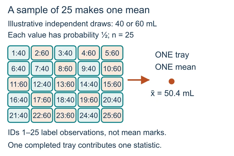Twenty-five labeled bottle values are combined into one sample-mean marker at 50.4 mL. Suppose each independent fill is equally likely to be 40 or 60 mL. This tray contains twelve 40-mL and thirteen 60-mL fills, totaling 1,260 mL; its 25 observations contribute one mean, 50.4 mL.

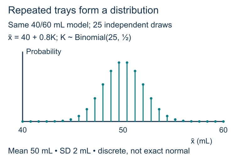Twenty-six possible sample means appear as discrete probability bars with a normal approximation drawn for comparison. For 25 independent fills equally likely to be 40 or 60 mL, K is binomial with n = 25 and p = 0.5, and the tray mean is 40 + 0.8K. The exact distribution is discrete, centered at 50 mL with standard deviation 2 mL. A normal curve approximates its shape.

SECTION 4

Mathematical Framework

The behavior of sampling distributions is governed by a small set of elegant results. These formulas quantify the center, spread, and shape of the distribution of common statistics, transforming an intuitive idea into a precise tool for inference.

MEAN OF THE SAMPLING DISTRIBUTION OF x̄

μ_{x̄} = μ

The mean of the sampling distribution of x̄ equals the population mean μ. This confirms that x̄ is an unbiased estimator of μ — on average, the sample mean hits the target.

STANDARD ERROR OF x̄

σ_{x̄} = σ / √n

The standard error measures how much x̄ varies from sample to sample. It decreases with the square root of the sample size n, meaning that quadrupling n cuts the standard error in half.

MEAN OF THE SAMPLING DISTRIBUTION OF p̂

μ_{p̂} = p

For a sample proportion p̂, the center of its sampling distribution equals the true population proportion p. Like x̄, p̂ is unbiased.

STANDARD ERROR OF p̂

σ_{p̂} = √[ p(1 − p) / n ]

The variability of p̂ depends on both the true proportion p and the sample size n. The spread is maximized when p = 0.5 and decreases as p moves toward 0 or 1, reflecting the reduced uncertainty when events are rare or near-certain.

ℹ

The 10% Condition

SECTION 5

The Effect of Sample Size on Variability

One of the most important insights in statistics is that increasing the sample size reduces sampling variability. The relationship is not linear — the standard error decreases proportionally to 1/√n, producing diminishing returns. Moving from n = 25 to n = 100 halves the standard error, but moving from n = 100 to n = 400 is required to halve it again. The diagram below compares three sampling distributions for x̄ with the same population but different sample sizes, illustrating this tightening effect.

Three bell curves share the same center (μ = 100) but differ in spread. The orange curve (n = 10) is widest, the violet curve (n = 30) is narrower, and the cyan curve (n = 100) is tightest, illustrating the σ/√n relationship.

Sample Size (n)	Standard Error σ_{x̄}	Relative Width
10	30/√10 ≈ 9.49	Widest — high variability
25	30/√25 = 6.00	Moderate
100	30/√100 = 3.00	Narrow — low variability
400	30/√400 = 1.50	Narrowest — very low variability

Standard error for σ = 30 across several sample sizes

★

Key takeaway

DIMINISHING RETURNS

SECTION 6

Worked Example: Describing a Sampling Distribution

Suppose a large university reports that the mean time students spend studying per week is μ = 14 hours with a standard deviation of σ = 6 hours. A researcher takes a simple random sample of n = 36 students. Describe the sampling distribution of the sample mean x̄ and find the probability that x̄ exceeds 16 hours.

Worked example

1
Step 1 — Identify the Parameter and Given Values

The population mean is μ = 14 hours and the population standard deviation is σ = 6 hours. The sample size is n = 36. We are asked about the sampling distribution of x̄.
2
Step 2 — Check Conditions

The university is described as "large," so the total student population N is well above 360. Since n = 36 ≤ 0.10N, the 10% condition is satisfied, and we may treat observations as approximately independent. Additionally, since n = 36 ≥ 30, the Central Limit Theorem ensures the sampling distribution of x̄ is approximately normal regardless of the population shape.
3
Step 3 — Compute the Mean of the Sampling Distribution

By the unbiasedness property, μ_{x̄} = μ = 14 hours.

μ_{x̄} = 14 hours
4
Step 4 — Compute the Standard Error

The standard error is σ_{x̄} = σ / √n = 6 / √36 = 6 / 6 = 1 hour.

σ_{x̄} = 1 hour
5
Step 5 — State the Sampling Distribution

The sampling distribution of x̄ is approximately Normal with mean 14 and standard deviation 1. In notation: x̄ ~ N(14, 1).
6
Step 6 — Compute the Probability P(x̄ > 16)

Convert to a z-score: z = (16 − 14) / 1 = 2. Using the standard normal table or calculator, P(Z > 2) = 1 − 0.9772 = 0.0228.

P(x̄ > 16) ≈ 0.0228 (about 2.3%)
7
Step 7 — Interpret in Context

If the true mean study time is 14 hours, there is only about a 2.3% chance that a random sample of 36 students would produce a sample mean above 16 hours. This low probability would lead us to question whether μ = 14 is correct if we did observe x̄ > 16 — this reasoning is the foundation of hypothesis testing.

SECTION 7

Bias vs. Variability: What Can Go Wrong?

A good estimator must satisfy two criteria: it should be centered on the parameter (low bias) and it should not scatter too widely (low variability). Sampling variability is an inherent consequence of working with samples and can be reduced by increasing n. Bias, on the other hand, is a systematic tendency for the estimator to miss the parameter in one direction, and it cannot be fixed by increasing sample size alone — it requires changing the sampling method. A voluntary response survey, for example, is biased because the respondents are self-selected; no amount of additional voluntary responses will fix the distortion.

Characteristic	Bias	Variability
Definition	The sampling distribution is centered away from the true parameter.	The statistic scatters widely across different samples.
Source	Flawed sampling design (convenience, voluntary response, undercoverage).	Random chance inherent in drawing a sample.
Fixed by larger n?	No — bias persists regardless of sample size.	Yes — standard error decreases as n grows.
Remedy	Use probability-based sampling: SRS, stratified, cluster designs.	Increase the sample size n.
Dartboard analogy	Darts consistently land to the left of the bullseye.	Darts scatter widely around the bullseye.

Bias vs. Variability comparison

★

Key takeaway

THE IDEAL ESTIMATOR

SECTION 8

Connection to the Central Limit Theorem and Inference

The ideas in this lesson — that statistics vary from sample to sample, that their variability is quantifiable, and that sampling distributions have predictable shapes — are not ends in themselves. They are the scaffolding upon which all of statistical inference is built. The Central Limit Theorem (CLT) formalizes what we have hinted at: for sufficiently large n, the sampling distribution of x̄ is approximately normal regardless of the population's shape. This normality is what makes z-scores and t-scores viable tools for constructing confidence intervals and performing hypothesis tests.

Concept	This Lesson (Introduction)	Next Steps (CLT & Inference)
Focus	Why do different samples give different results?	What exact shape does the sampling distribution take, and how do we use it?
Key formula	σ_{x̄} = σ / √n	z = (x̄ − μ) / (σ / √n) and the t-statistic when σ is unknown
Shape assumption	Approximately normal for large n (informal)	CLT provides the formal justification and conditions
Application	Describing variability and checking conditions	Confidence intervals and hypothesis tests

This lesson vs. where the course is headed

Keep in mind that sampling distributions also apply to other statistics: the sample proportion p̂, the difference of two means (x̄₁ − x̄₂), and the difference of two proportions (p̂₁ − p̂₂). In every case, the same logic applies: identify the center, compute the spread using the appropriate standard error formula, verify the conditions for normality, and then use the resulting model to make probability statements. Mastering this reasoning now will make every subsequent inference topic feel like a natural extension of the same framework.

SECTION 9

Practice Problems

Question 1: CONCEPTUAL

A polling organization takes a simple random sample of 500 likely voters and records the proportion who favor a ballot initiative. If the organization were to repeat this process with a new simple random sample of 500 from the same population, which of the following is the best explanation for why the two sample proportions would most likely differ?

A. The polling organization made a measurement error in at least one of the surveys.
B. The population proportion changed between the two surveys.
C. Random selection means each sample includes different individuals, producing natural sampling variability.
D. A sample of 500 is too small to produce consistent results.
E. The sampling method was biased, causing the proportions to shift.

Show answer (C)

C is correct. Sampling variability arises because each random sample includes a different set of individuals, and so the sample proportion p̂ naturally fluctuates from sample to sample. A is incorrect because the question describes a straightforward polling process with no mention of measurement error; the difference is expected even with perfect measurement. B is incorrect because the question states the same population is being sampled; the parameter is assumed fixed. D is incorrect because n = 500 is a reasonably large sample; even very large samples exhibit sampling variability — it just becomes smaller. E is incorrect because the problem specifies a simple random sample, which is an unbiased sampling method.

Question 2: BASIC CALCULATION

A population has mean μ = 80 and standard deviation σ = 20. A simple random sample of n = 64 observations is drawn. What is the standard error of the sample mean x̄?

A. 0.3125
B. 1.25
C. 2.50
D. 5.00
E. 20.00

Show answer (C)

C is correct. The standard error is σ_{x̄} = σ / √n = 20 / √64 = 20 / 8 = 2.50. A (0.3125) would result from dividing σ by n instead of √n (20/64). B (1.25) would result from dividing σ by n and then multiplying by 4, suggesting a computational error. D (5.00) would result from using √n = √16 instead of √64, perhaps confusing n with n/4. E (20.00) is the population standard deviation σ itself — this is the spread of individual observations, not the spread of x̄.

Question 3: INTERMEDIATE

In a certain city, 35% of households have at least one dog (p = 0.35). A researcher selects a simple random sample of 200 households from the city's 50,000 households. Which of the following correctly describes the sampling distribution of the sample proportion p̂?

A. Approximately Normal with mean 0.35 and standard deviation 0.0337
B. Approximately Normal with mean 0.35 and standard deviation 0.2275
C. Approximately Normal with mean 70 and standard deviation 6.75
D. Approximately Normal with mean 0.35 and standard deviation 0.0011
E. The Normal approximation cannot be used because the 10% condition is not satisfied.

Show answer (A)

A is correct. First, check conditions. 10% condition: n = 200 ≤ 0.10 × 50,000 = 5,000, satisfied. Large counts: np = 200(0.35) = 70 ≥ 10 and n(1 − p) = 200(0.65) = 130 ≥ 10, satisfied. So p̂ is approximately Normal with mean μ_{p̂} = p = 0.35 and standard deviation σ_{p̂} = √[0.35(0.65)/200] = √[0.2275/200] = √0.001138 ≈ 0.0337. B uses p(1 − p) = 0.2275 without dividing by n. C describes the distribution of the count (np = 70), not the proportion p̂. D computes p(1 − p)/n but forgets to take the square root. E is incorrect because 200 is well under 10% of 50,000.

Question 4: APPLIED

4 pts

A quality control manager at a bottling plant knows that the fill amounts of bottles follow a distribution with mean μ = 500 mL and standard deviation σ = 8 mL. Every hour, the manager takes a random sample of n = 16 bottles and computes the sample mean fill amount x̄. (a) Describe the sampling distribution of x̄. State the mean and standard error. (b) The manager flags the process if x̄ falls below 496 mL. Find the probability that the process is flagged when the process is operating correctly (μ = 500). (c) The manager considers increasing the sample size to n = 64. How would this change the probability computed in part (b)? Explain without performing a full calculation. (d) Explain why using a larger sample makes the quality control procedure more effective.

Show answer

Part (a) — 1 point: The sampling distribution of x̄ has mean μ_{x̄} = 500 mL and standard error σ_{x̄} = σ/√n = 8/√16 = 2 mL. Since n = 16 and the population distribution is not stated to be normal, a note about the CLT or an assumption of approximate normality should be included. If the population is approximately normal, then x̄ ~ N(500, 2). Part (b) — 1 point: z = (496 − 500)/2 = −2. P(x̄ < 496) = P(Z < −2) = 0.0228. There is approximately a 2.28% chance the process is flagged when it is operating correctly. Part (c) — 1 point: With n = 64, the standard error would decrease to σ/√64 = 1 mL, which is half the original standard error. The z-score for 496 would become (496 − 500)/1 = −4, which corresponds to a much smaller probability. The probability of a false flag would decrease substantially (from about 0.0228 to approximately 0.00003). Part (d) — 1 point: A larger sample reduces the standard error of x̄, making the sampling distribution more tightly concentrated around the true mean. This means that when the process is operating correctly, x̄ is very unlikely to fall below the threshold (fewer false alarms). Conversely, when the process genuinely shifts away from 500 mL, the tighter distribution makes it more likely that x̄ will cross the threshold (better detection). Thus, a larger sample improves the procedure's ability to distinguish between a correctly functioning process and a malfunctioning one.

Question 5: CRITICAL THINKING

4 pts

Two AP Statistics students each independently collect a simple random sample of 40 students from their large high school to estimate the mean number of hours spent on extracurricular activities per week. Student A obtains x̄ = 6.2 hours and Student B obtains x̄ = 7.8 hours. (a) Explain why it is expected that Student A and Student B obtained different sample means, even though they sampled from the same population. (b) Suppose the true population mean is μ = 7.0 hours and σ = 4.0 hours. Compute the standard error of x̄ and use it to assess whether the difference between the two sample means (7.8 − 6.2 = 1.6 hours) is surprisingly large. (c) A third student collects a sample of n = 160 from the same population. Would you expect this student's sample mean to be closer to μ = 7.0 than the first two? Justify your answer using the concept of the sampling distribution. (d) Explain why neither Student A's nor Student B's result is "wrong." In what sense does the sampling distribution provide the framework for evaluating individual sample results?

Show answer

Part (a) — 1 point: Different sample means are expected because of sampling variability. Each simple random sample includes a different set of 40 students, and the particular individuals selected influence the computed mean. This variation is a natural and unavoidable consequence of random sampling, not an indication of error or bias. Part (b) — 1 point: The standard error is σ_{x̄} = 4.0/√40 ≈ 0.632 hours. The difference between the two sample means is 1.6 hours. Because the two samples are independent, the standard error of the difference x̄_B − x̄_A is √(0.632² + 0.632²) ≈ 0.894 hours. The z-score for the difference is 1.6/0.894 ≈ 1.79, which corresponds to a two-tailed p-value of about 0.073. This means a difference of 1.6 hours or more would occur roughly 7.3% of the time by chance alone — somewhat unusual but not extremely rare. Individually,

z_A

= (6.2 − 7.0)/0.632 ≈ −1.27 and

z_B

= (7.8 − 7.0)/0.632 ≈ 1.27, so neither sample mean is extreme on its own. Part (c) — 1 point: Yes. With n = 160, the standard error decreases to 4.0/√160 ≈ 0.316 hours, which is half the standard error for n = 40. The sampling distribution of x̄ for the third student is more tightly concentrated around μ = 7.0, so it is more likely that this student's sample mean will fall close to 7.0. In general, the probability that x̄ falls within any fixed distance of μ increases as the sample size increases. Part (d) — 1 point: Neither result is wrong because both are plausible outcomes from the sampling distribution of x̄ when μ = 7.0. The sampling distribution tells us the full range of values x̄ could take and how likely each range is. Any individual sample mean is just one realization from this distribution. Rather than judging a single sample as correct or incorrect, we use the sampling distribution to quantify how unusual the result is under a given assumption about μ. This is the conceptual basis for inference: we do not expect any single sample to perfectly capture the parameter, but the sampling distribution provides the probability model that allows us to measure and communicate our uncertainty.