Expected Counts in Two-Way Tables - AP Statistics

SECTION 1

Historical Context & Motivation

Understanding the relationship between two categorical variables has been a central challenge in statistical analysis since the nineteenth century. When a researcher asks whether smoking status is associated with lung disease, or whether political affiliation differs across age groups, the raw counts in a two-way table (also called a contingency table) provide the starting point. However, observed counts alone cannot tell us whether a pattern is statistically meaningful or merely the product of random variation. To answer that question, we need a benchmark — a set of counts that represents what we would see if the two variables had no association at all. These benchmarks are called expected counts, and they form the theoretical backbone of every chi-square test for independence and homogeneity.

1900 • Pearson's Chi-Square

Karl Pearson introduced the chi-square goodness-of-fit test, establishing the formal comparison of observed and expected frequencies as a pillar of inferential statistics.

1922 • Fisher's Exact Test

Ronald Fisher developed an exact test for 2 × 2 tables, underscoring the need for well-defined expected counts even when sample sizes are small.

1954 • Cochran's Guidelines

William Cochran formalized the rule that expected counts should generally be at least 5 in each cell to ensure the chi-square approximation is reliable.

2000s • Modern AP Curriculum

Expected counts became a standard topic in the AP Statistics framework, appearing in both the chi-square test for independence and the chi-square test for homogeneity.

The central question expected counts address is deceptively simple: If two categorical variables were completely independent, how many observations would fall into each cell of a two-way table? Answering this question precisely is what allows us to measure the discrepancy between what we observe and what independence predicts, ultimately powering the chi-square statistic.

SECTION 2

Core Principles & Definitions

Before computing expected counts, it is essential to internalize several foundational ideas that connect probability theory to the structure of contingency tables. These principles ensure you understand not just how to calculate expected counts but why the formula works.

Independence Assumption

Two categorical variables are independent if knowing the value of one provides no information about the other. Under independence, joint probabilities equal the product of marginal probabilities: P(A ∩ B) = P(A) × P(B).

Marginal Totals

The row totals and column totals of a two-way table are called marginal totals. They represent the univariate distributions of each variable separately and are treated as fixed when computing expected counts.

Expected Count Formula

For any cell in row i and column j, the expected count equals (row i total × column j total) ÷ grand total. This distributes the grand total proportionally across cells under the assumption of independence.

Not Necessarily Integers

Expected counts are theoretical averages, not actual counts. They can be — and usually are — non-integer values such as 14.67 or 8.25. Never round expected counts to whole numbers for chi-square calculations.

Validity Condition

The chi-square approximation is considered valid when all expected counts are at least 5. If any expected count falls below 5, consider combining categories or using Fisher's exact test.

✦

KEY TAKEAWAY

Think of expected counts as the blueprint for a perfectly balanced factory. If a candy company produces 60% milk chocolate and 40% dark chocolate, and independently packages 70% in small bags and 30% in large bags, you would expect 42% of all packages to be milk-chocolate-in-small-bags (0.60 × 0.70 = 0.42). Expected counts simply scale that proportion up to the total number of items observed. Any deviation from this blueprint is the signal the chi-square test evaluates.

SECTION 3

Visual Explanation

The following diagram illustrates a complete two-way table for a study examining the relationship between exercise frequency (Low, Moderate, High) and health outcome (Healthy, Unhealthy). Observed counts are shown in each cell alongside their row and column marginal totals. The diagram highlights how each cell's expected count derives from its corresponding row total and column total divided by the grand total.

The dashed lines trace how the row total (150, cyan), column total (80, violet), and grand total (250, amber) feed into the expected count formula for the Healthy-Low cell, yielding an expected count of 48.0.

In the diagram above, notice that the observed count for the Healthy-Low cell is 30, but the expected count under independence is 48. This discrepancy is precisely the kind of deviation the chi-square test measures. Each cell's expected count preserves the marginal distributions: the expected values in the Healthy row still sum to 150, and those in the Low column still sum to 80, ensuring overall consistency with the data's structure.

SECTION 4

Mathematical Framework

The expected count formula is a direct consequence of the multiplication rule for independent events. If the row variable and column variable are independent, then the probability that a randomly selected observation falls in row i and column j equals the product of the marginal probabilities. Multiplying that joint probability by the grand total gives the expected count.

INDEPENDENCE CONDITION

P(Row i ∩ Col j) = P(Row i) × P(Col j)

Under the null hypothesis of independence, the joint probability of being in row i and column j equals the product of the two marginal probabilities.

EXPECTED COUNT FORMULA

E_ij = (R_i × C_j) / n

Where E_ij = expected count for row i and column j, R_i = total for row i, C_j = total for column j, and n = grand total of all observations.

To see why this formula works, consider that P(Row i) is estimated by R_i / n and P(Col j) is estimated by C_j / n. Under independence, the expected proportion in cell (i, j) is (R_i / n) × (C_j / n). Multiplying by n yields (R_i × C_j) / n, which is the standard formula. This derivation makes clear that expected counts allocate the grand total across cells in exact proportion to the marginal distributions.

CHI-SQUARE TEST STATISTIC

χ² = Σ (O_ij − E_ij)² / E_ij

The chi-square statistic sums the squared differences between observed (O_ij) and expected (E_ij) counts, each divided by the expected count, over all cells. Larger values indicate greater departure from independence.

DEGREES OF FREEDOM

df = (r − 1)(c − 1)

Where r = number of rows and c = number of columns. For a 2 × 3 table, df = (2 − 1)(3 − 1) = 2.

SECTION 5

Building the Complete Expected-Count Table

Returning to our exercise-and-health example, let us compute the expected count for every cell and display the full table side by side with the observed counts. This comparison provides immediate visual insight into which cells contribute most to the chi-square statistic. When computing expected counts, always use unrounded intermediate values; rounding prematurely introduces error that compounds in the chi-square calculation.

The left table shows observed counts, the right table shows expected counts under independence (pink). Every calculation uses the same formula: (row total × column total) / grand total. All six expected counts exceed 5, satisfying the validity condition for the chi-square test.

💡

Consistency Check

Always verify that your expected counts sum correctly: each row of expected counts should sum to the original row total, each column should sum to the original column total, and the overall sum should equal the grand total. For example, 48.0 + 48.0 + 54.0 = 150 (Healthy row total) and 48.0 + 32.0 = 80 (Low column total). If these checks fail, you have a computation error.

SECTION 6

Worked Example

A university admissions office wants to investigate whether admission status (Admitted, Denied) is associated with the applicant's intended major (Engineering, Business, Liberal Arts). A random sample of 400 applicants yields the following observed counts.

	Engineering	Business	Liberal Arts	Row Total
Admitted	80	60	100	240
Denied	40	60	60	160
Col Total	120	120	160	400

Observed counts for admission status vs. intended major

Computing Expected Counts & Chi-Square Statistic

1
Step 1 — Identify Marginal Totals

Row totals: Admitted = 240, Denied = 160. Column totals: Engineering = 120, Business = 120, Liberal Arts = 160. Grand total n = 400.
2
Step 2 — Compute Expected Counts

Apply E_ij = (R_i × C_j) / n for each cell. Admitted-Engineering: (240 × 120)/400 = 72. Admitted-Business: (240 × 120)/400 = 72. Admitted-Liberal Arts: (240 × 160)/400 = 96. Denied-Engineering: (160 × 120)/400 = 48. Denied-Business: (160 × 120)/400 = 48. Denied-Liberal Arts: (160 × 160)/400 = 64.

Expected counts: 72, 72, 96, 48, 48, 64 — all ≥ 5 ✓
3
Step 3 — Verify Marginal Sums

Admitted row: 72 + 72 + 96 = 240 ✓. Denied row: 48 + 48 + 64 = 160 ✓. Engineering column: 72 + 48 = 120 ✓. Business column: 72 + 48 = 120 ✓. Liberal Arts column: 96 + 64 = 160 ✓.
4
Step 4 — Compute Chi-Square Contributions

For each cell, compute (O − E)² / E. Admitted-Eng: (80 − 72)² / 72 = 64/72 ≈ 0.889. Admitted-Bus: (60 − 72)² / 72 = 144/72 = 2.000. Admitted-LA: (100 − 96)² / 96 = 16/96 ≈ 0.167. Denied-Eng: (40 − 48)² / 48 = 64/48 ≈ 1.333. Denied-Bus: (60 − 48)² / 48 = 144/48 = 3.000. Denied-LA: (60 − 64)² / 64 = 16/64 = 0.250.
5
Step 5 — Sum and Interpret

χ² = 0.889 + 2.000 + 0.167 + 1.333 + 3.000 + 0.250 = 7.639. Degrees of freedom: (2 − 1)(3 − 1) = 2. Using a chi-square distribution with df = 2, the p-value is approximately 0.022. At α = 0.05, we reject the null hypothesis and conclude that there is statistically significant evidence of an association between admission status and intended major.

χ² = 7.639, df = 2, p ≈ 0.022 → Reject H₀ at α = 0.05

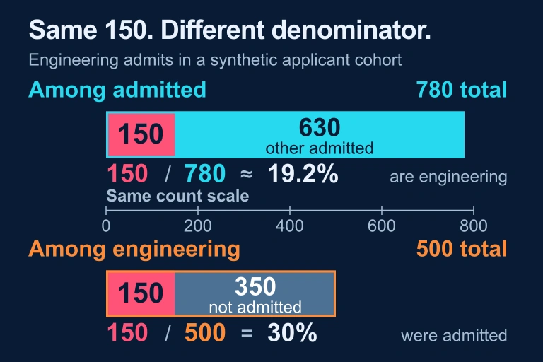
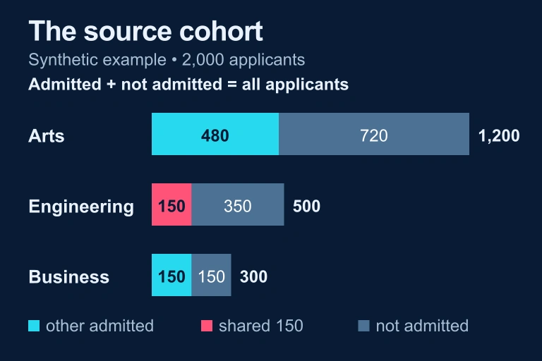The same 150 admitted engineering applicants compared with denominators 780 admitted applicants and 500 engineering applicants, giving about 19.2% and 30%.

Applicant cohorts of 1200,500,300 with admitted counts 480,150,150 and other counts 720,350,150.

Separate 2,000-applicant illustration: an expected count here is 500×780/2000=195. Preserve the original 400-observation table with expected rows [72,72,96] and [48,48,64].

SECTION 7

Common Pitfalls & Exam Tips

Common Pitfall	Why It's Wrong	Correct Approach
Using observed counts in the denominator of the χ² formula	The formula divides by expected counts, not observed counts. Using observed counts changes the distribution of the test statistic.	Always divide (O − E)² by E, the expected count.
Rounding expected counts to whole numbers	Expected counts are theoretical values and need not be integers. Premature rounding introduces unnecessary error.	Keep at least two decimal places throughout all calculations.
Ignoring the validity condition	If any expected count is below 5, the χ² distribution is a poor approximation, and the p-value may be unreliable.	State that all expected counts are ≥ 5 as part of your conditions check on the AP exam.
Confusing the test for independence with the test for homogeneity	Both use the same χ² formula and expected count calculation, but the sampling designs differ (one sample vs. separate samples from each population).	Identify the study design first. Hypotheses and calculations remain the same; interpretation and context differ.
Computing expected counts using proportions from the sample instead of the formula	While conceptually equivalent, manually multiplying proportions increases the risk of rounding error compared to the direct formula.	Use E = (Row Total × Column Total) / Grand Total directly.

Common mistakes and corrections for expected count calculations

📋

AP EXAM STRATEGY

On the AP Statistics exam, every chi-square free-response question requires you to check conditions before running the test. The expected count condition (all expected counts ≥ 5) must be verified explicitly — simply stating the condition without showing the actual expected counts will not earn full credit. Think of expected counts as the structural inspection before building a house: skip it, and the entire framework is suspect. Present your expected counts in a clearly labeled table or list, then state: "All expected counts are at least 5, so the chi-square approximation is appropriate."

SECTION 8

Connection to Advanced Topics

Expected counts in two-way tables form the gateway to a broader family of chi-square procedures and advanced categorical analysis. Understanding expected counts thoroughly prepares you not only for the AP exam but also for more sophisticated methods you may encounter in college-level statistics or data science coursework.

Feature	Expected Counts (AP Level)	Advanced Extensions
Table size	r × c tables with moderate cell counts	Multi-way tables (3+ variables) analyzed via log-linear models
Small expected counts	Combine categories or note violation	Fisher's exact test, simulation-based tests, or exact conditional inference
Effect size	Chi-square statistic and p-value	Cramér's V, phi coefficient, standardized residuals for individual cells
Model complexity	Test for independence or homogeneity	Logistic regression, generalized linear models for categorical response
Interpretation focus	Is there an association? (yes/no)	Which specific cells deviate most? What is the nature and direction of the association?

AP-level expected counts vs. advanced categorical analysis

One particularly useful extension is the concept of standardized residuals, defined as (O − E) / √E for each cell. While the AP exam focuses on the overall χ² statistic, standardized residuals allow researchers to pinpoint which specific cells contribute most to a significant result. A standardized residual exceeding ±2 suggests that particular cell deviates substantially from what independence predicts — a technique that bridges the gap between the simple hypothesis test and deeper exploratory analysis of categorical data.

SECTION 9

Practice Problems

Question 1: CONCEPTUAL

A researcher constructs a two-way table with three rows and four columns. Which of the following best describes what an expected count represents for a particular cell?

A. The number of observations actually recorded in that cell from the sample data.
B. The count that would appear in the cell if the two categorical variables were perfectly correlated.
C. The count that would appear in the cell if the two categorical variables were independent, given the observed marginal totals.
D. The mean of the observed counts across all cells in the table.
E. The count obtained by evenly distributing the grand total across all 12 cells.

Show answer (C)

C is correct. An expected count represents the theoretical count in a cell under the null hypothesis of independence between the two categorical variables, calculated using the marginal totals. A is wrong because it describes the observed count, not the expected count. B is wrong because expected counts assume independence (no association), not perfect correlation. D is wrong because expected counts are cell-specific, computed from the product of the relevant row and column totals divided by the grand total — not a simple grand mean. E is wrong because equal distribution ignores the marginal structure; expected counts respect the differing row and column totals.

Question 2: BASIC CALCULATION

In a two-way table, a particular cell is in a row whose total is 90 and a column whose total is 60. The grand total is 300. What is the expected count for this cell?

A. 15
B. 18
C. 25
D. 30
E. 50

Show answer (B)

B is correct. Using the formula E = (Row Total × Column Total) / Grand Total = (90 × 60) / 300 = 5400 / 300 = 18. A (15) would result from an incorrect calculation such as (90 × 50)/300. C (25) might come from dividing the grand total by the number of cells in a certain table, ignoring marginal structure. D (30) could result from simply dividing the row total by 3 without using the column total. E (50) bears no systematic relationship to the correct computation.

Question 3: INTERMEDIATE

A 3 × 2 two-way table has a grand total of 200. One cell has an observed count of 28 and an expected count of 35. What is the contribution of this cell to the chi-square statistic?

A. 0.25
B. 1.00
C. 1.40
D. 1.75
E. 7.00

Show answer (C)

C is correct. The contribution of a single cell to χ² is (O − E)² / E = (28 − 35)² / 35 = (−7)² / 35 = 49 / 35 = 1.40. A (0.25) would result from dividing the difference (7) by the observed count and not squaring. B (1.00) might arise from dividing (O − E)² by 49 instead of 35. D (1.75) could come from dividing 49 by 28 (the observed count instead of the expected count). E (7.00) is simply |O − E| without squaring or dividing — a common careless error.

Question 4: APPLIED

5 pts

A public health researcher surveys 500 adults and records their vaccination status (Vaccinated, Unvaccinated) and whether they contracted the flu that season (Yes, No). The observed two-way table is: Flu-Yes Flu-No Row Total Vaccinated: 30 270 300 Unvaccinated: 50 150 200 Col Total: 80 420 500 (a) Calculate the expected count for each of the four cells. (b) Verify that the expected counts satisfy the condition for a valid chi-square test. (c) Calculate the chi-square test statistic. (d) State the degrees of freedom and, using your calculator, determine the p-value. (e) At α = 0.05, state your conclusion in context.

Show answer

Rubric (5 points): Point 1 (Expected Counts): E(Vacc, Yes) = (300 × 80)/500 = 48. E(Vacc, No) = (300 × 420)/500 = 252. E(Unvacc, Yes) = (200 × 80)/500 = 32. E(Unvacc, No) = (200 × 420)/500 = 168. [1 point for correctly computing all four expected counts.] Point 2 (Conditions): All expected counts (48, 252, 32, 168) are at least 5, so the chi-square approximation is valid. [1 point for explicitly checking and stating the condition is satisfied.] Point 3 (Chi-Square Statistic): χ² = (30−48)²/48 + (270−252)²/252 + (50−32)²/32 + (150−168)²/168 = 324/48 + 324/252 + 324/32 + 324/168 = 6.75 + 1.286 + 10.125 + 1.929 = 20.089. [1 point for correct computation with work shown.] Point 4 (Degrees of Freedom and P-value): df = (2−1)(2−1) = 1. Using χ²cdf(20.089, ∞, 1) or equivalent, p-value ≈ 0.0000074, which is far less than 0.001. [1 point for correct df and valid p-value.] Point 5 (Conclusion in Context): Since p < 0.05, we reject the null hypothesis. There is convincing statistical evidence that vaccination status and flu contraction are associated among adults. Specifically, unvaccinated adults appear to contract the flu at a higher rate than expected under independence. [1 point for a conclusion that includes a decision, links to context, and references the p-value or significance level.]

Question 5: CRITICAL THINKING

4 pts

A sociologist collects data on political affiliation (Democrat, Republican, Independent) and opinion on a policy (Favor, Oppose) from 600 respondents. After computing expected counts, she finds that one cell has an expected count of 3.8. (a) Explain why this expected count is problematic for conducting a chi-square test. (b) Describe two different strategies the sociologist could use to address this problem. (c) Suppose the sociologist combines the Independent category with one of the other categories, resulting in a 2 × 2 table where all expected counts exceed 5. The chi-square test yields χ² = 0.42 with df = 1 and p = 0.517. Interpret this result in context. (d) A colleague argues that combining categories changes the research question. Evaluate this claim.

Show answer

Rubric (4 points): Point 1 (Explaining the problem): The chi-square test relies on the sampling distribution of the test statistic being approximately chi-square. This approximation requires all expected counts to be at least 5. An expected count of 3.8 violates this condition, which means the p-value obtained from the chi-square distribution may not accurately reflect the true probability of observing such a test statistic under the null hypothesis. The approximation tends to be poor when expected counts are small because the discrete distribution of cell counts does not closely match the continuous chi-square curve. [1 point] Point 2 (Two strategies): Strategy 1 — Combine categories. The sociologist could merge the Independent category with either Democrat or Republican (whichever is more conceptually sensible) to increase expected counts in all cells. Strategy 2 — Use Fisher's exact test (or a simulation-based approach). Rather than relying on the chi-square approximation, the sociologist could compute an exact p-value based on the hypergeometric distribution, which does not require any minimum expected count. Other valid strategies include collecting more data or using a randomization/permutation test. [1 point for describing two distinct, valid strategies.] Point 3 (Interpretation): With χ² = 0.42, df = 1, and p = 0.517, we fail to reject the null hypothesis at α = 0.05. There is not convincing statistical evidence of an association between political affiliation (as recoded into two groups) and opinion on the policy among the population of interest. The p-value of 0.517 means that if there were truly no association, we would observe a chi-square statistic of 0.42 or larger about 51.7% of the time, which is not unusual. [1 point for correct interpretation that includes context, a decision, and proper use of non-deterministic language.] Point 4 (Evaluating the claim): The colleague's concern is valid. The original research question examined three distinct political affiliations, and collapsing two categories into one fundamentally alters the comparison. For example, combining Independents with Democrats tests whether "Democrats-plus-Independents" differ from Republicans, which is a different hypothesis than whether the three groups differ from one another. Important nuances about Independent voters' opinions are lost. However, this trade-off may be necessary to meet the conditions for a valid test, and the researcher should acknowledge the limitation explicitly when reporting results. A preferable alternative might be Fisher's exact test, which preserves all three categories. [1 point for a substantive evaluation that addresses both the validity of the concern and the practical trade-off.]

SUMMARY

Summary

Expected counts represent the theoretical cell frequencies in a two-way table under the null hypothesis of independence between two categorical variables. They are computed using the formula E = (Row Total × Column Total) / Grand Total, which distributes the grand total across cells in exact proportion to the marginal distributions. Expected counts need not be integers, should never be rounded for calculations, and must each be at least 5 for the chi-square approximation to be valid.

The chi-square test statistic is computed as χ² = Σ (O − E)² / E, summing over all cells, and is compared to a chi-square distribution with df = (r − 1)(c − 1). On the AP exam, always verify the expected count condition explicitly, present your expected counts clearly, and interpret your results in the context of the problem. Mastering expected counts is essential for both the chi-square test for independence and the chi-square test for homogeneity.