

SECTION 1
Historical Context & Motivation
Many real-world probability questions resist clean, closed-form solutions. Combinatorial complexity, irregular sample spaces, and dependencies among events can make exact calculation extraordinarily difficult or even impossible. Simulation — the practice of using repeated random trials to approximate a probability — offers an empirical escape route. Rather than enumerating every outcome, we generate thousands (or millions) of random trials and observe how often the event of interest occurs. The resulting relative frequency converges toward the true probability as the number of trials grows, a principle grounded in the Law of Large Numbers. This idea has roots stretching back centuries, but it was the advent of modern computing that transformed simulation from a mathematical curiosity into an indispensable statistical tool.
1777 • Buffon's Needle Problem
1946 • The Monte Carlo Method
1979 • Random Number Generators in Curricula
2000s • Simulation in AP Statistics
The central question this lesson addresses is deceptively simple: How can we estimate a probability that is difficult or impossible to compute exactly? By designing an appropriate random mechanism, running many trials, and computing relative frequencies, we obtain an estimate that improves with the number of repetitions. Understanding how to set up, conduct, and interpret a simulation is a foundational skill tested on the AP Statistics exam.
SECTION 2
Core Principles & Definitions
Before designing a simulation, it is essential to internalize several foundational ideas that govern why and how simulation works. Each principle connects the abstract notion of probability to the concrete act of generating random outcomes.
Law of Large Numbers
Random Number Generation
Model Component Mapping
Trial and Response Variable
Variability & Repetition
KEY TAKEAWAY
SECTION 3
Visualizing Convergence in Simulation
The diagram below illustrates the core insight behind simulation: as the number of trials increases, the cumulative relative frequency converges toward the true theoretical probability. Early in the process the estimate fluctuates wildly, but by several hundred trials it stabilizes within a narrow band around the true value.
Notice how after approximately 200 trials, the simulated relative frequency rarely deviates by more than 0.03 from the true probability. This diminishing fluctuation is not a coincidence; it reflects the theoretical result that the standard deviation of the sample proportion decreases proportionally to 1/√n. Doubling your trials does not double precision — it improves it by a factor of √2 ≈ 1.41. This is why simulation studies often use thousands or even tens of thousands of repetitions to achieve high accuracy.
SECTION 4
Mathematical Framework
Although simulation is an empirical technique, its reliability rests on well-established mathematical foundations. The key equations below formalize the relationship between the number of trials, the estimated probability, and the precision of that estimate.
ESTIMATED PROBABILITY
where X = number of trials in which event A occurred, and n = total number of simulation trials. This is simply the relative frequency of event A.
LAW OF LARGE NUMBERS
The empirical relative frequency P̂(A) converges in probability to the true probability P(A) as the number of trials grows without bound.
STANDARD DEVIATION OF SIMULATED PROPORTION
This formula quantifies the precision of a simulation estimate. When the true probability is near 0.5 and n = 1000, the standard deviation is √(0.25/1000) ≈ 0.016, meaning about 95% of simulation estimates will fall within ±0.032 of the true probability.
These equations reveal an important design consideration: the required number of simulation trials depends on the desired precision. If you need your estimate to be accurate within ±0.01 with 95% confidence, you can solve 2 × √(0.25/n) ≤ 0.01, yielding n ≥ 10,000 trials. For most AP exam contexts, a few hundred to a few thousand trials are sufficient because the exam focuses on the process of designing the simulation rather than demanding extreme numerical precision.
SECTION 5
Designing a Simulation: Step-by-Step Process
Every simulation on the AP Statistics exam follows a structured four-step process. Mastering this framework ensures that your free-response answers earn full credit, because the scoring rubric rewards clear articulation of each step. The flowchart below visualizes how these steps connect.
Detailed Step Descriptions
In Step 1, you choose a random device and create a correspondence between its outcomes and the real-world event. For example, if a basketball player makes 70% of free throws, you might let digits 0–6 represent a made shot and digits 7–9 represent a miss using randInt(0,9). The key is that the proportions of digits assigned must match the given probabilities. If the probability is something like 1/3, you could use digits 1–3 for success and 4–9 plus 0 for failure (not all 10 digits are used equally, so you might use a three-digit scheme or simply let 1–3 = success, 4–9 = failure, and 0 = skip/redo).
In Step 2, you specify what constitutes one complete trial. If you are simulating 5 consecutive free throws, one trial consists of generating 5 random digits — each representing one shot attempt. Be explicit: state the number of random digits generated per trial and what stopping rule applies.
In Step 3, you define the response variable — the outcome you record after each trial. This might be "Did the player make at least 4 out of 5 shots? (yes/no)" or "How many shots until the first miss?" The response variable directly connects to the probability question being asked.
In Step 4, you repeat the trial many times and compute the estimated probability as the number of "successes" divided by the total number of trials. On a calculator, you might use a loop to automate 1000 repetitions. On the AP exam, you might perform a small number of trials by hand using a random digit table and then state that in practice you would use many more trials.
SECTION 6
Worked Example: Simulating a Cereal Box Prize Collection
A cereal company places one of 5 different prizes (equally likely) inside each box. You want to estimate the probability that a customer collects all 5 different prizes by purchasing exactly 10 boxes. This problem is difficult to solve analytically (it involves inclusion-exclusion with Stirling numbers), but a simulation provides a quick estimate.
Cereal Prize Simulation
- 1
Step 1 — Define the Random Device
Each box contains one of 5 equally likely prizes. UserandInt(1,5)on a calculator, where each digit 1 through 5 represents one specific prize. Alternatively, using a random digit table, let digits 1–5 represent the five prizes and ignore digits 0 and 6–9 (since the prizes are equally likely with probability 1/5 each, and digits 1–5 each appear with probability 1/10 among the used digits, but each has the same probability, so the conditional distribution given a valid digit is uniform).randInt(1,5) maps uniformly to the 5 prizes. - 2
Step 2 — Define One Trial
One trial consists of generating 10 random integers between 1 and 5 (inclusive), representing 10 cereal box purchases. Each of the 10 numbers represents the prize found in that box.One trial = 10 random integers from {1, 2, 3, 4, 5}. - 3
Step 3 — Define the Response Variable
After generating the 10 numbers, count the number of distinct values. If all 5 distinct values (1, 2, 3, 4, 5) appear at least once in the set of 10 numbers, record the trial as a "success." Otherwise, record it as a "failure."Success = all 5 distinct prizes appear among the 10 boxes. - 4
Step 4 — Run Trials and Estimate
Suppose we run 1000 trials using a calculator or computer. A sample run of 5 trials using the random digit table might produce: Trial 1: 3 1 5 2 4 1 3 5 2 4 → all 5 present → Success Trial 2: 2 2 1 3 1 2 5 3 1 2 → missing 4 → Failure Trial 3: 5 4 3 2 1 5 4 3 2 1 → all 5 present → Success Trial 4: 1 1 2 2 3 3 4 4 5 5 → all 5 present → Success Trial 5: 3 3 2 1 4 2 3 1 4 2 → missing 5 → Failure In 5 hand trials: 3 successes out of 5, giving P̂ = 3/5 = 0.60. With 1000 computer-generated trials, suppose 522 trials result in all 5 prizes being collected.P̂(all 5 prizes in 10 boxes) = 522/1000 = 0.522 - 5
Step 5 — Interpret
Based on the simulation, we estimate that the probability of collecting all 5 different prizes in exactly 10 box purchases is approximately 0.52. The exact theoretical probability is 5! × S(10,5) / 5¹⁰ ≈ 0.522, so the simulation estimate is very close. Note that with only 5 hand trials, the estimate of 0.60 was noticeably off — reinforcing the need for many repetitions.Estimated probability ≈ 0.52 (close to the exact value of ≈ 0.522).
AP Exam Tip
 Collecting all prize types and waiting for the first designated prize use different stopping rules. Define the response variable before generating trials.
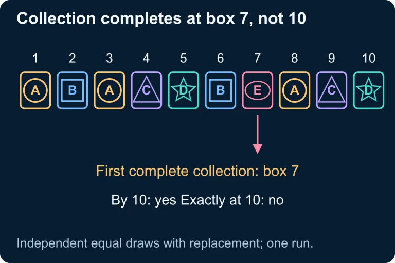 Suppose each box independently contains one of five equally likely prize types. In the sequence A, B, A, C, D, B, E, A, C, D, all five types first appear at box 7. This trial succeeds for completion by ten boxes; repeated trials estimate the event’s probability.
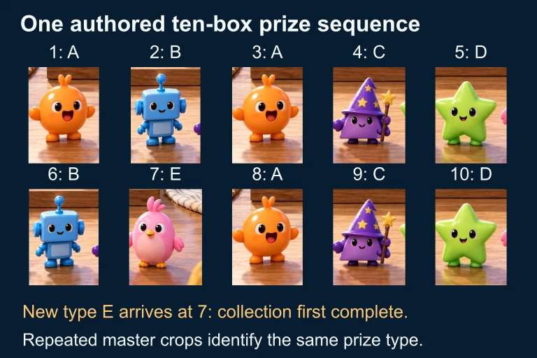 The ten-box sequence is A, B, A, C, D, B, E, A, C, D. New types increase the collection count; repeated types leave it unchanged. Start a fresh collection for the next trial.
SECTION 7
Strengths & Limitations of Simulation
Simulation is an extraordinarily flexible tool, but like any method it comes with trade-offs. Understanding these strengths and limitations helps you decide when simulation is the right approach and how to interpret its results responsibly.
| Aspect | Strengths | Limitations |
|---|---|---|
| Complexity | Can handle problems with complex dependencies, irregular sample spaces, and multiple stages that resist closed-form solutions. | Results are only estimates, not exact answers. Rare events (P < 0.001) require enormous numbers of trials to estimate accurately. |
| Accessibility | Requires no advanced mathematical derivation. Students with basic probability knowledge can design and run simulations. | Setting up the random device incorrectly — for example, using the wrong probability assignments — produces systematically biased results. |
| Reproducibility | Setting a random seed allows exact reproduction of results, facilitating verification and collaboration. | Different random seeds yield different estimates. Results always carry sampling variability that must be acknowledged. |
| Scalability | Computers can execute millions of trials in seconds, making simulation practical for complex real-world scenarios. | Hand simulation with random digit tables is slow and error-prone, limiting the number of trials in exam settings. |
Strengths and limitations of simulation as a probability estimation method.
KEY TAKEAWAY
SECTION 8
Connection to Inference & Advanced Methods
Simulation as introduced in this lesson forms the conceptual bedrock for more sophisticated statistical methods you will encounter later in AP Statistics and in college-level courses. The same logic — generating random outcomes to build a distribution — underpins randomization tests, permutation tests, and bootstrap confidence intervals. Understanding simulation now prepares you to think computationally about inference.
| Feature | Basic Simulation (This Lesson) | Advanced Methods (Later Topics) |
|---|---|---|
| Purpose | Estimate a single probability P(A) | Build entire sampling distributions, compute p-values, construct confidence intervals |
| Null model | Random device mirrors known probabilities in the scenario | Random device mimics the null hypothesis (e.g., no treatment effect) |
| Output | A single number: P̂(A) | A distribution of simulated statistics used for inference |
| Assumptions | Probabilities and independence structure are known | May relax distributional assumptions; resampling from observed data |
| AP Exam Context | Unit 4: Probability | Units 6–9: Inference for proportions, means, regression |
How basic simulation connects to advanced statistical inference methods.
In a randomization test, for example, you simulate the test statistic thousands of times under the assumption that the null hypothesis is true, then compare the observed statistic to that simulated null distribution to compute a p-value. The four-step process you learned in this lesson — define the device, define a trial, define the response, repeat and analyze — carries over directly. Mastering it now provides a conceptual framework that makes parametric inference (z-tests, t-tests, chi-square tests) more intuitive when you encounter those topics later.
SECTION 9
Practice Problems
Question 1: CONCEPTUAL
- A. The assignment gives girls a probability of 5/10 = 0.50, which correctly matches the assumption of equally likely.
- B. The student should use only digits 0–1 (for girl and boy) and ignore 2–9.
- C. Four digits per trial is not enough to estimate the probability accurately.
- D. There is no serious flaw; the simulation design is valid.
- E. The student must use a computer rather than a random digit table for the simulation to be valid.
Show answer (D)
Question 2: BASIC CALCULATION
- A. P̂ = 0.156; this is very close to the theoretical probability of 1/6 ≈ 0.167.
- B. P̂ = 0.156; this is significantly different from the theoretical probability of 1/12 ≈ 0.083.
- C. P̂ = 0.078; this is very close to the theoretical probability of 1/12 ≈ 0.083.
- D. P̂ = 0.780; the simulation greatly overestimates the theoretical probability.
- E. P̂ = 0.156; this is very close to the theoretical probability of 7/36 ≈ 0.194.
Show answer (A)
Question 3: INTERMEDIATE
- A. 00–39 = Red, 40–74 = Blue, 75–99 = Green
- B. 00–40 = Red, 41–75 = Blue, 76–99 = Green
- C. 01–40 = Red, 41–74 = Blue, 75–99 and 00 = Green
- D. 1–4 = Red, 5–7 = Blue, 8–0 = Green (single digits)
- E. 00–39 = Red, 40–69 = Blue, 70–99 = Green
Show answer (A)
Question 4: APPLIED
4 ptsShow answer
Question 5: CRITICAL THINKING
4 ptsShow answer
SUMMARY
Lesson Summary
Summary
Simulation is a powerful empirical method for estimating probabilities that are difficult or impossible to compute exactly. The approach relies on the Law of Large Numbers, which guarantees that the relative frequency of an event converges to its true probability as the number of trials increases. Every simulation follows a structured four-step process: (1) define the random device with correct probability assignments, (2) define one trial, (3) define the response variable, and (4) repeat many trials and compute P̂(A) = X/n.
On the AP Statistics exam, clearly describing each step in context is essential for earning full rubric credit. More trials yield more precise estimates, with the standard deviation of the simulated proportion decreasing as 1/√n. Simulation connects directly to randomization-based inference methods encountered later in the course, making it a foundational skill that bridges probability and statistical inference.