Carrying Out a Test for the Difference of Two Population Proportions - AP Statistics

SECTION 1

Historical Context & Motivation

Comparing proportions across two groups is one of the most common tasks in applied research. Whether a medical team wants to know if a new vaccine reduces infection rates relative to a placebo, or a marketing analyst asks whether an email redesign lifts click-through rates, the underlying statistical question is the same: do the two population proportions p₁ and p₂ differ? The formal machinery for answering this question grew out of more than a century of work in probability theory, normal approximation, and hypothesis testing.

1733 • De Moivre's Normal Approximation

Abraham de Moivre showed that the binomial distribution could be approximated by the normal curve for large samples, laying the foundation for z-based inference on proportions.

1900 • Pearson's Chi-Square Test

Karl Pearson introduced the chi-square goodness-of-fit test, providing a general framework for comparing observed and expected categorical frequencies—closely related to comparing two proportions.

1925 • Fisher & Neyman–Pearson Frameworks

Ronald Fisher formalized significance testing, while Jerzy Neyman and Egon Pearson later introduced the concepts of Type I error, Type II error, and power, giving hypothesis testing its modern structure.

1970s–Present • Modern Curriculum & AP Statistics

The two-proportion z-test became a standard topic in introductory courses and the AP Statistics exam, reflecting its central role in evidence-based decision making across disciplines.

The central question this lesson addresses is straightforward yet powerful: given sample data from two independent groups, how do we formally test whether the difference in their sample proportions provides convincing evidence that the corresponding population proportions are truly different? Answering that question requires a pooled estimate, a test statistic, and a p-value—each of which we will develop step by step.

SECTION 2

Core Principles & Definitions

Before computing anything, it is essential to understand the conceptual building blocks of the two-proportion z-test. The test compares two independent groups on a single binary outcome—success or failure—and asks whether any observed difference in sample proportions is large enough to rule out chance as a plausible explanation.

Null & Alternative Hypotheses

The null hypothesis states H₀: p₁ − p₂ = 0 (no difference). The alternative can be two-sided (≠) or one-sided (< or >), depending on the research question.

Pooled Proportion (p̂_c)

Under H₀ the two populations share a common proportion, so we combine both samples to get a single pooled estimate: p̂_c = (X₁ + X₂) / (n₁ + n₂), where X₁ and X₂ are the counts of successes.

Standard Error (Pooled)

The standard error of p̂₁ − p̂₂ under H₀ uses the pooled proportion: SE = √[ p̂_c(1 − p̂_c)(1/n₁ + 1/n₂) ]. This measures how much the difference in sample proportions would vary across repeated samples if H₀ were true.

Test Statistic (z)

z = (p̂₁ − p̂₂) / SE. This standardized value tells us how many standard errors the observed difference lies from zero. Under H₀ and large-sample conditions, z follows approximately a standard normal distribution.

P-Value & Decision

The p-value is the probability of obtaining a test statistic as extreme as (or more extreme than) the observed z, assuming H₀ is true. If p-value ≤ α, we reject H₀ and conclude there is convincing evidence of a difference.

SECTION 3

Visual Explanation — The Testing Procedure

The flowchart above summarizes the six-step procedure for a two-proportion z-test. Each box represents one stage—from stating hypotheses through the final contextual conclusion. In Sections 4 and 6 we expand on the computation in Steps 3–5.

The flowchart reinforces a critical point: the computation of the test statistic (Step 4) depends on the pooled proportion, which is only appropriate when we assume H₀: p₁ = p₂. If you were instead constructing a confidence interval for p₁ − p₂, you would use unpooled standard error—a distinction worth remembering on exam day.

SECTION 4

Mathematical Framework

The two-proportion z-test rests on the sampling distribution of p̂₁ − p̂₂. When both samples are sufficiently large and drawn independently, the Central Limit Theorem guarantees that p̂₁ − p̂₂ is approximately normal. Under H₀: p₁ − p₂ = 0, the mean of this distribution is 0 and we estimate its standard deviation with the pooled standard error.

POOLED PROPORTION

p̂_c = (X₁ + X₂) / (n₁ + n₂)

X₁ and X₂ are the number of successes in samples 1 and 2; n₁ and n₂ are the respective sample sizes. This single proportion is our best estimate of the common p under H₀.

POOLED STANDARD ERROR

SE = √[ p̂_c (1 − p̂_c) (1/n₁ + 1/n₂) ]

This expression combines the variability from both samples. The factor (1/n₁ + 1/n₂) captures that larger samples yield smaller standard errors.

TEST STATISTIC

z = (p̂₁ − p̂₂ − 0) / SE

We subtract 0 because the hypothesized difference under H₀ is zero. The resulting z follows approximately the standard normal distribution N(0, 1) when conditions are met.

P-VALUE

Two-sided: p-value = 2 × P(Z ≥ |z|) One-sided: p-value = P(Z ≥ z) or P(Z ≤ z)

Z is a standard normal random variable. Use the direction indicated by Hₐ. On the AP exam, you may use a calculator's 2-PropZTest function or Table A.

ℹ

Conditions Checklist

SECTION 5

Sampling Distribution & Condition Details

Understanding why conditions matter requires visualizing the sampling distribution of p̂₁ − p̂₂ under the null hypothesis. When H₀ is true, the distribution is centered at 0 with a spread determined by the pooled standard error. The diagram below illustrates how the observed difference maps onto this distribution to produce a p-value.

The bell curve (violet) represents the sampling distribution of p̂₁ − p̂₂ under H₀, centered at 0. The red dot marks the observed z-value. The shaded tails represent the two-sided p-value—the probability of getting a test statistic at least this extreme in either direction.

Why Each Condition Matters

Condition	What Could Go Wrong	How to Verify
Random	Without randomness, sampling bias may make p̂₁ and p̂₂ unrepresentative, invalidating any inference.	Confirm random sampling (observational study) or random assignment (experiment) in the problem stem.
Independence (10%)	Dependent observations produce a smaller true SE than assumed, inflating the z-statistic and yielding spurious significance.	Check n₁ ≤ 0.10 × N₁ and n₂ ≤ 0.10 × N₂, or note random assignment in an experiment (which guarantees independence).
Large Counts	If expected counts are too small, the normal approximation is poor and the stated p-value may be inaccurate.	Verify n₁p̂_c ≥ 10, n₁(1−p̂_c) ≥ 10, n₂p̂_c ≥ 10, n₂(1−p̂_c) ≥ 10 using the pooled proportion.

Three conditions for the two-proportion z-test

SECTION 6

Worked Example

A researcher randomly assigns 250 patients to receive a new drug and 250 patients to receive a placebo. In the drug group, 180 out of 250 show symptom improvement. In the placebo group, 155 out of 250 show improvement. At α = 0.05, is there convincing evidence that the drug produces a higher improvement rate than the placebo?

Worked example

1
Step 1 — State Hypotheses

Let p₁ = the true proportion who improve with the drug and p₂ = the true proportion who improve with the placebo. H₀: p₁ − p₂ = 0 (no difference). Hₐ: p₁ − p₂ > 0 (the drug is better). This is a one-sided test (right-tailed).
2
Step 2 — Check Conditions

Random: Patients were randomly assigned to treatment groups. ✓ Independent: Random assignment supports the treatment comparison. The z-test also assumes independent individual responses and no material clustering or interference; these conditions must be justified by the study design. Large Counts: We need p̂_c first (computed in Step 3): p̂_c = 0.67. Then n₁p̂_c = 250 × 0.67 = 167.5 ≥ 10, n₁(1−p̂_c) = 82.5 ≥ 10, n₂p̂_c = 167.5 ≥ 10, n₂(1−p̂_c) = 82.5 ≥ 10. ✓ The large-count condition is met; the analysis is conditional on the independence assumptions above.
3
Step 3 — Compute Pooled Proportion

p̂₁ = 180/250 = 0.72. p̂₂ = 155/250 = 0.62. The pooled proportion is:

p̂_c = (180 + 155) / (250 + 250) = 335 / 500 = 0.67
4
Step 4 — Compute Standard Error

SE = √[ 0.67 × 0.33 × (1/250 + 1/250) ] = √[ 0.2211 × 0.008 ] = √0.001769

SE ≈ 0.04206
5
Step 5 — Compute Test Statistic

z = (p̂₁ − p̂₂) / SE = (0.72 − 0.62) / 0.04206 = 0.10 / 0.04206

z ≈ 2.377
6
Step 6 — Find P-Value

Since Hₐ is one-sided (>), the p-value = P(Z ≥ 2.377). Using the standard normal table or calculator: p-value ≈ 0.0087.

p-value ≈ 0.0087
7
Step 7 — State Conclusion in Context

Conditional on those study-design assumptions, because the p-value (0.0087) is less than α = 0.05, we reject H₀. There is convincing evidence that the proportion of patients who improve is higher for the drug group than for the placebo group.

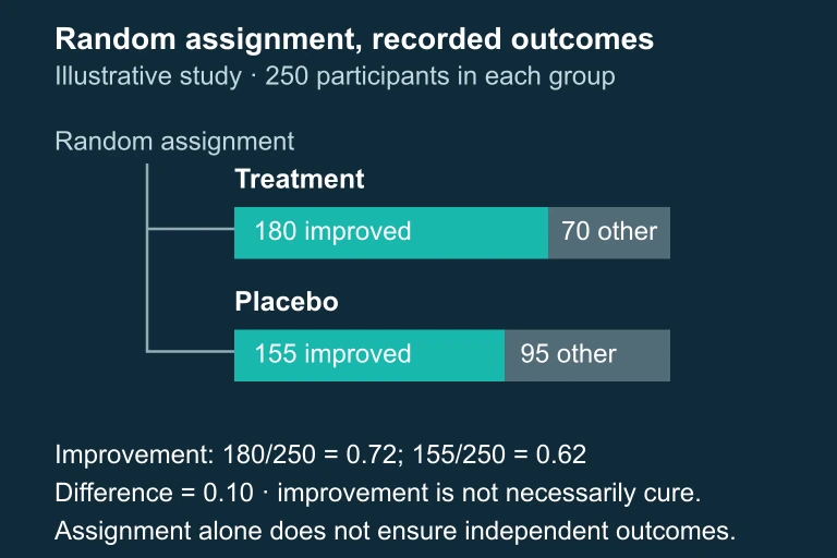Random assignment to two groups of 250, with 180 improved and 70 not improved in one group, and 155 improved and 95 not improved in the other. Proportions are 0.72 and 0.62. The assigned treatment and placebo groups have observed improvement fractions 0.72 and 0.62; random assignment does not by itself guarantee independent outcomes.

SECTION 7

Common Errors & Exam Pitfalls

Mistake	Why It's Wrong	Correct Approach
Using unpooled SE in the hypothesis test	Under H₀ both populations share one proportion; using separate p̂ values overestimates or underestimates SE.	Always use the pooled proportion p̂_c for the SE in a significance test.
Using pooled SE in a confidence interval	A CI does not assume H₀ is true, so pooling is inappropriate.	Use unpooled SE = √[ p̂₁(1−p̂₁)/n₁ + p̂₂(1−p̂₂)/n₂ ] for CIs.
Checking Large Counts with p̂₁ and p̂₂ separately	The conditions for the test require expected counts under H₀, which means using p̂_c.	Verify all four: n₁p̂_c, n₁(1−p̂_c), n₂p̂_c, n₂(1−p̂_c) ≥ 10.
Generic conclusion not linked to context	AP rubrics require a conclusion stated in terms of the problem's variables and scenario.	Mention the populations, the variable, and use non-definitive language ('convincing evidence').
Confusing 'fail to reject H₀' with 'accept H₀'	We never prove H₀ true; we only say the data do not provide sufficient evidence against it.	Write: 'We do not have convincing evidence that p₁ ≠ p₂.'

Common exam-day errors and how to avoid them

SECTION 8

Connection to Chi-Square & Advanced Methods

The two-proportion z-test is closely related to the chi-square test of homogeneity. In fact, for a two-sided test comparing two proportions, the chi-square statistic with 1 degree of freedom equals z² exactly. The z-test, however, has the advantage of supporting one-sided alternatives and directly producing a signed test statistic that indicates the direction of the difference. As you advance, you will encounter logistic regression, which generalizes proportion comparisons to multiple predictors, and Fisher's exact test, which handles very small samples where the normal approximation fails.

Feature	Two-Proportion z-Test	Chi-Square Test of Homogeneity
Number of groups	Exactly 2	2 or more
One-sided Hₐ possible?	Yes	No (always two-sided)
Test statistic	z (standard normal)	χ² (chi-square with df = (r−1)(c−1))
Relationship	z² = χ² when df = 1 and Hₐ is two-sided	Generalizes the z-test to multi-group settings
When to prefer	Directional hypotheses or when you need a CI	Comparing 3+ groups or when direction is not specified

Two-proportion z-test vs. chi-square test of homogeneity

Looking ahead, techniques such as logistic regression allow researchers to compare proportions while controlling for confounding variables—something the simple z-test cannot do. Mastering the two-proportion z-test builds the conceptual foundation you will need for these more advanced methods.

SECTION 9

Practice Problems

Question 1: CONCEPTUAL

When carrying out a two-proportion z-test, why do we use a pooled proportion rather than the individual sample proportions to compute the standard error?

A. Because pooling always reduces Type I error regardless of the hypothesis.
B. Because the null hypothesis assumes both populations share a common proportion, so combining the samples gives the best estimate of that shared value for the SE calculation.
C. Because using separate proportions would make the z-statistic too large.
D. Because pooling is required by the Central Limit Theorem.
E. Because pooled and unpooled standard errors always give the same test statistic.

Show answer (B)

Under the null hypothesis H₀: p₁ = p₂, we assume both populations share a single common proportion. The pooled proportion p̂_c combines the data from both samples to produce the best estimate of that shared parameter. Using separate sample proportions would contradict the null hypothesis we are testing, because it would treat the two populations as having different proportions even while we are evaluating whether they differ.

Question 2: BASIC CALCULATION

In a study, 84 out of 200 subjects in Group A and 60 out of 200 subjects in Group B experienced an event. What is the pooled proportion p̂_c?

A. 0.42
B. 0.30
C. 0.36
D. 0.72
E. 0.21

Show answer (C)

p̂_c = (84 + 60) / (200 + 200) = 144 / 400 = 0.36. Choice C is correct because we simply add the successes and divide by the total sample size. Choice A (0.42) is the proportion for Group A alone. Choice B (0.30) is the proportion for Group B alone. Choice D (0.72) doubles the correct answer. Choice E (0.21) appears to use an incorrect denominator.

Question 3: INTERMEDIATE

A poll of 400 adults from City X found 52% support a policy, while a poll of 500 adults from City Y found 45% support it. Using α = 0.05 and a two-sided alternative, which of the following is closest to the test statistic z?

A. 0.70
B. 1.40
C. 1.87
D. 2.09
E. 2.63

Show answer (D)

First, compute p̂_c = (0.52×400 + 0.45×500) / (400 + 500) = (208 + 225) / 900 = 433/900 ≈ 0.4811. SE = √[0.4811 × 0.5189 × (1/400 + 1/500)] = √[0.24964 × 0.0045] = √0.001123 ≈ 0.03352. z = (0.52 − 0.45) / 0.03352 = 0.07 / 0.03352 ≈ 2.09. Choice D is correct. Choice A (0.70) results from omitting the square root. Choice B (1.40) uses an incorrect SE. Choice C (1.87) miscalculates the pooled proportion. Choice E (2.63) uses unpooled SE.

Question 4: APPLIED

A technology company randomly assigns 600 users to a new app interface (Group A) and 600 users to the current interface (Group B). After one week, 258 users in Group A completed a key action, compared to 216 in Group B. Carry out a full two-proportion z-test at α = 0.05 to determine whether the new interface produces a higher completion rate. State hypotheses, check conditions, compute the test statistic and p-value, and state your conclusion in context.

Show answer

Hypotheses: Let p₁ = the true proportion completing the action under the new interface and p₂ = the same under the current interface. H₀: p₁ − p₂ = 0; Hₐ: p₁ − p₂ > 0. Conditions: Random — users were randomly assigned. ✓ Independent — random assignment guarantees independence between groups. ✓ Large Counts — p̂_c = (258 + 216)/(600 + 600) = 474/1200 = 0.395. n₁p̂_c = 237 ≥ 10, n₁(1−p̂_c) = 363 ≥ 10, n₂p̂_c = 237 ≥ 10, n₂(1−p̂_c) = 363 ≥ 10. ✓ Computation: p̂₁ = 258/600 = 0.43, p̂₂ = 216/600 = 0.36. SE = √[0.395 × 0.605 × (1/600 + 1/600)] = √[0.23898 × 0.003333] = √0.000797 ≈ 0.02823. z = (0.43 − 0.36)/0.02823 = 0.07/0.02823 ≈ 2.48. P-value = P(Z ≥ 2.48) ≈ 0.0066. Conclusion: Because the p-value (≈ 0.0066) is less than α = 0.05, we reject H₀. There is convincing evidence that the new app interface produces a higher completion rate than the current interface.

Question 5: CRITICAL THINKING

A researcher tests H₀: p₁ = p₂ versus Hₐ: p₁ ≠ p₂ and obtains z = 1.80 with a two-sided p-value of 0.0718 at α = 0.05. She fails to reject H₀. Her colleague argues that because the one-sided p-value (0.0359) is below 0.05, they should switch to a one-sided test and reject H₀. (a) Explain why this reasoning is flawed. (b) Describe a scenario in which a one-sided test would have been legitimate from the outset. (c) A 95% confidence interval for p₁ − p₂ is (−0.005, 0.145). Explain how this interval is consistent with failing to reject H₀, and discuss what it tells us about the practical significance of the difference.

Show answer

(a) Switching from a two-sided to a one-sided test after seeing the data is a form of data-snooping (sometimes called p-hacking). The choice of Hₐ must be determined before looking at results; otherwise, the true Type I error rate exceeds the stated α. The researcher effectively halves her significance threshold only in the favorable direction, which inflates false-positive risk. (b) A one-sided test would be legitimate if, prior to data collection, the research question specifically asked whether p₁ > p₂ based on theory, prior studies, or the structure of the intervention (e.g., 'Does the new treatment improve outcomes compared to the control?'). The directionality must be justified by context, not by the observed data. (c) The 95% CI (−0.005, 0.145) contains 0, which is consistent with failing to reject H₀ at α = 0.05 in the two-sided test—a CI that includes the null value corresponds to a non-rejection. However, the interval is almost entirely positive, suggesting the true difference may be positive but is too imprecisely estimated to confirm. The upper bound of 0.145 indicates the difference could be as large as about 14.5 percentage points, which may be practically meaningful. A larger sample size could narrow this interval and potentially allow the researcher to detect a meaningful difference if one exists.