Conditional Probability - AP Statistics

SECTION 1

Historical Context & Motivation

The idea that new information should update our beliefs about uncertain events is so intuitive that people have practiced it informally for millennia—gamblers adjusted their bets, physicians revised diagnoses, and navigators re-estimated positions as data arrived. Yet formalizing this intuition into a rigorous mathematical framework required centuries of intellectual effort. Conditional probability provides the precise language for answering the question: given that some event has occurred, how does that knowledge change the probability of another event? This deceptively simple question sits at the heart of modern statistics, machine learning, medical testing, and forensic science.

1654 • Pascal & Fermat Correspondence

Blaise Pascal and Pierre de Fermat exchanged letters on the "problem of points," laying the groundwork for probability theory by analyzing how partial information about a game's progress affects the fair division of stakes.

1713 • Bernoulli's Ars Conjectandi

Jacob Bernoulli's posthumous work systematized combinatorial probability and introduced the law of large numbers, establishing the theoretical soil in which conditional reasoning would later take root.

1763 • Bayes' Theorem Published

Thomas Bayes' essay, published posthumously by Richard Price, presented the first formal method for inverting conditional probabilities—computing P(cause | effect) from P(effect | cause). This became the cornerstone of Bayesian inference.

1812 • Laplace's Théorie Analytique

Pierre-Simon Laplace independently derived and extended Bayes' result, applying conditional probability to problems ranging from celestial mechanics to the reliability of witness testimony, popularizing its use across the sciences.

1933 • Kolmogorov's Axioms

Andrey Kolmogorov published his axioms of probability, within which conditional probability received a rigorous measure-theoretic definition, unifying the classical, frequentist, and Bayesian perspectives under one framework.

The central question that conditional probability addresses is straightforward yet profound: if we restrict our attention to only those outcomes where event B has already happened, what fraction of that restricted sample space does event A occupy? Mastering this concept equips you to tackle Bayes' theorem, independence testing, and the probability distributions that form the backbone of the AP Statistics curriculum.

SECTION 2

Core Principles & Definitions

Before computing any conditional probabilities, it is essential to ground yourself in the foundational ideas that make the concept coherent. Conditional probability is not a separate species of probability; rather, it is the ordinary probability measure applied to a reduced sample space. When you learn that event B has occurred, the original sample space S effectively shrinks to B, and every probability must be re-scaled accordingly.

Sample Space Reduction

Conditioning on B replaces the original sample space S with B itself. Only outcomes inside B remain possible, so all probabilities are recalculated relative to P(B).

The Conditional Formula

P(A | B) = P(A ∩ B) / P(B), provided P(B) > 0. This ratio captures the proportion of B-outcomes that also belong to A.

Multiplication Rule

Rearranging the formula gives P(A ∩ B) = P(B) × P(A | B). This is the general multiplication rule, valid whether or not A and B are independent.

Independence Connection

Events A and B are independent if and only if P(A | B) = P(A). Learning that B occurred does not change the probability of A—knowing B provides no information about A.

Asymmetry of Conditioning

P(A | B) ≠ P(B | A) in general. Confusing these two is the "inverse fallacy" or "prosecutor's fallacy," a common error in everyday reasoning and even in courtrooms.

✦

KEY TAKEAWAY

Think of conditional probability like a filter on a spreadsheet. Imagine a dataset with 1,000 rows. The unconditional probability P(A) counts all rows satisfying A out of 1,000. Conditioning on B is equivalent to applying a filter that keeps only the rows where B is true—say 200 rows remain. Now P(A | B) counts how many of those 200 filtered rows also satisfy A. You have not changed the data; you have merely narrowed your focus, which is exactly what the formula P(A ∩ B) / P(B) accomplishes algebraically.

SECTION 3

Visual Explanation — Venn Diagram Perspective

A Venn diagram offers the most accessible visual model for conditional probability. In the diagram below, the entire rectangle represents the sample space S, circle A represents event A, and circle B represents event B. The overlap region is the intersection A ∩ B. When we condition on B, we conceptually discard everything outside circle B and ask: what proportion of circle B's area is occupied by the shaded intersection?

The pink-shaded intersection represents P(A ∩ B). When we condition on B, the cyan circle becomes our entire universe, and the conditional probability P(A | B) equals the ratio of the shaded region to the full area of circle B.

Notice that the Venn diagram makes the asymmetry of conditioning visually obvious. If you instead conditioned on A—making circle A your new universe—the ratio would be the intersection area divided by the total area of circle A, which in general differs from the earlier ratio. This visual intuition is invaluable on the AP exam, where many free-response questions ask you to justify your probability computations by referencing an appropriate diagram or two-way table.

SECTION 4

Mathematical Framework

The algebraic machinery of conditional probability is compact but remarkably powerful. From a single definition, you can derive the multiplication rule, the law of total probability, and Bayes' theorem—three results that together form the engine of probabilistic inference.

DEFINITION OF CONDITIONAL PROBABILITY

P(A | B) = P(A ∩ B) / P(B), P(B) > 0

P(A | B) is read "the probability of A given B." P(A ∩ B) is the joint probability that both A and B occur. P(B) is the marginal probability of the conditioning event.

GENERAL MULTIPLICATION RULE

P(A ∩ B) = P(B) × P(A | B) = P(A) × P(B | A)

This rule follows directly by rearranging the conditional probability definition. It generalizes to chains of events: P(A ∩ B ∩ C) = P(A) × P(B | A) × P(C | A ∩ B).

LAW OF TOTAL PROBABILITY

P(A) = P(A | B₁)P(B₁) + P(A | B₂)P(B₂) + ⋯ + P(A | Bₙ)P(Bₙ)

Here B₁, B₂, …, Bₙ form a partition of S (mutually exclusive and exhaustive). This formula lets you compute P(A) by breaking the sample space into manageable pieces.

BAYES' THEOREM

P(B | A) = P(A | B) × P(B) / P(A)

Bayes' theorem "reverses" the conditioning direction. P(B) is the prior probability, P(A | B) is the likelihood, and P(B | A) is the posterior probability. P(A) in the denominator is often expanded using the law of total probability.

💡

Independence Shortcut

When A and B are independent, P(A | B) = P(A), so the multiplication rule simplifies to P(A ∩ B) = P(A) × P(B). On the AP exam, always verify independence before using this shortcut—state the condition explicitly to earn full credit on free-response questions.

SECTION 5

Detailed Breakdown — Two-Way Tables & Tree Diagrams

While the Venn diagram offers geometric intuition, the two most practical tools for computing conditional probabilities on the AP exam are the two-way frequency table and the tree diagram. A two-way table organizes counts (or relative frequencies) for two categorical variables, making joint, marginal, and conditional probabilities immediately readable. A tree diagram, on the other hand, visually encodes sequential conditioning and is especially useful for problems involving the multiplication rule or Bayes' theorem.

	Tested Positive (T⁺)	Tested Negative (T⁻)	Total
Has Disease (D)	72	8	80
No Disease (D')	45	875	920
Total	117	883	1,000

Hypothetical medical screening results for 1,000 patients

From this table, conditional probabilities are extracted by restricting to a single row or column. For instance, P(D | T⁺) = 72 / 117 ≈ 0.615—among those who tested positive, only about 61.5% actually have the disease. Conversely, P(T⁺ | D) = 72 / 80 = 0.90, which is the test's sensitivity. Confusing these two quantities—P(D | T⁺) versus P(T⁺ | D)—is a classic instance of the inverse fallacy and a frequent source of lost points on the AP exam.

Each branch of the tree multiplies probabilities along its path to produce joint probabilities at the leaves. To find P(D | T⁺) via Bayes' theorem, divide the D ∩ T⁺ leaf (0.072) by the sum of all T⁺ leaves (0.072 + 0.045 = 0.117), yielding 0.072 / 0.117 ≈ 0.615.

The tree diagram makes the multiplication rule visually explicit: you multiply along each path from root to leaf to obtain joint probabilities. To apply Bayes' theorem, you sum the leaf values that correspond to your observed evidence (here, all T⁺ leaves) and then divide the specific leaf of interest by that sum. This "multiply along, add across" strategy is one of the most efficient techniques you can deploy on the AP exam.

SECTION 6

Worked Example

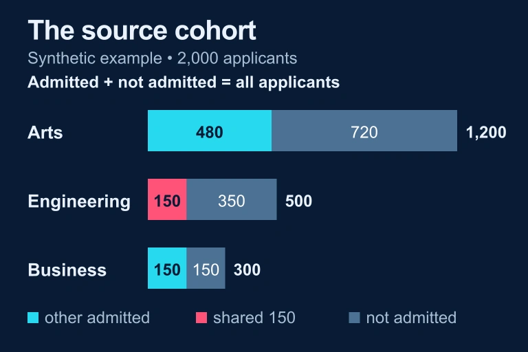
A university admissions office reports the following data for 2,000 applicants: 60% applied to the College of Arts & Sciences (A), 25% applied to the School of Engineering (E), and 15% applied to the School of Business (B). Among Arts & Sciences applicants, 40% were admitted; among Engineering applicants, 30% were admitted; and among Business applicants, 50% were admitted. A randomly selected applicant is found to have been admitted. What is the probability that this student applied to Engineering?

Bayes' Theorem — Admissions Scenario

1
Step 1 — Identify Given Information

Let A, E, and B denote the events of applying to Arts & Sciences, Engineering, and Business respectively. Let W denote the event of being admitted ("winning" admission). We are given: P(A) = 0.60, P(E) = 0.25, P(B) = 0.15, P(W | A) = 0.40, P(W | E) = 0.30, P(W | B) = 0.50.
2
Step 2 — Compute Joint Probabilities (Multiply Along)

Apply the multiplication rule to each branch: P(A ∩ W) = 0.60 × 0.40 = 0.24, P(E ∩ W) = 0.25 × 0.30 = 0.075, P(B ∩ W) = 0.15 × 0.50 = 0.075.

Joint probabilities: 0.24, 0.075, 0.075
3
Step 3 — Find P(W) Using the Law of Total Probability (Add Across)

P(W) = P(A ∩ W) + P(E ∩ W) + P(B ∩ W) = 0.24 + 0.075 + 0.075 = 0.39. So 39% of all applicants were admitted.

P(W) = 0.39
4
Step 4 — Apply Bayes' Theorem

P(E | W) = P(E ∩ W) / P(W) = 0.075 / 0.39 ≈ 0.1923. Among admitted students, approximately 19.2% applied to Engineering.

P(E | W) ≈ 0.192
5
Step 5 — Interpret in Context

Although 25% of all applicants chose Engineering, only about 19.2% of admitted students came from Engineering. This makes sense because Engineering had the lowest admit rate (30%), so it is under-represented among admitted students relative to its share of the applicant pool.

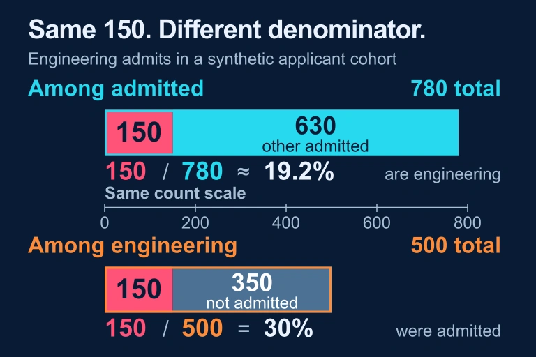
The same 150 admitted engineering applicants compared with denominators 780 admitted applicants and 500 engineering applicants, giving about 19.2% and 30%.

Applicant cohorts of 1200,500,300 with admitted counts 480,150,150 and other counts 720,350,150.

💡

AP Exam Tip

Free-response questions require you to show your work and communicate your reasoning in context. Always name the events, state the rule you are using (e.g., "By Bayes' theorem…" or "Using the general multiplication rule…"), show the arithmetic, and interpret your final answer in the language of the problem—don't just leave a number.

A screening station routes positive results into two different origins. A positive screening result can come from someone with or without the condition. Conditioning on a positive result changes the denominator to all positive results.

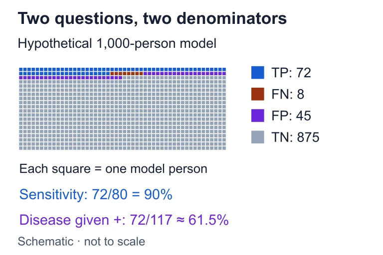
A 1,000-person grid partitions 72 true positives, 8 false negatives, 45 false positives and 875 true negatives, highlighting different conditional denominators. Suppose 1,000 people include 72 true positives, 8 false negatives, 45 false positives and 875 true negatives. Sensitivity is 72/80 = 90%. Among the 117 positive results, 72 have the condition, so P(condition | positive) = 72/117 ≈ 61.5%.

SECTION 7

Common Errors & Pitfalls

Conditional probability is conceptually elegant but operationally treacherous. Students lose points on the AP exam not because the formulas are difficult, but because the language of "given" is easy to misinterpret and the temptation to confuse related quantities is strong. The table below catalogs the most frequent errors and pairs each with a corrective strategy.

Error	Description	Corrective Strategy
Inverse Fallacy	Confusing P(A \| B) with P(B \| A). For example, assuming P(disease \| positive test) equals P(positive test \| disease).	Always write the full conditional notation. Ask yourself: which event is the given (the denominator)? Use Bayes' theorem to invert if needed.
Assuming Independence	Multiplying P(A) × P(B) without verifying that A and B are independent. This can lead to incorrect joint probabilities.	Use the general multiplication rule P(A ∩ B) = P(A) × P(B \| A) unless independence is explicitly stated or can be verified from the data.
Wrong Denominator	Using the total sample size rather than the conditioning event's count when reading from a two-way table.	When computing P(A \| B), restrict to the row or column for B first. Your denominator is the marginal total for B, not the grand total.
Confusing Disjoint and Independent	Believing that mutually exclusive events are independent. In fact, if A and B are disjoint and both have positive probability, they are dependent because P(A \| B) = 0 ≠ P(A).	Remember: disjoint means they cannot co-occur; independent means they do not influence each other. These are logically incompatible for events with nonzero probability.

✦

KEY TAKEAWAY

The most reliable way to avoid errors with conditional probability is to build a complete probability model before computing anything. Whether you choose a two-way table, a tree diagram, or a Venn diagram with filled-in values, having the full joint distribution in front of you makes it nearly impossible to grab the wrong denominator or confuse the conditioning direction. On the AP exam, the two minutes spent constructing the model will save you from costly mistakes.

SECTION 8

Connection to Advanced Theory

Conditional probability is not merely a topic within probability—it is arguably the organizing principle of modern statistical inference. Every confidence interval, hypothesis test, and regression model implicitly involves conditioning: we condition on the observed data to make statements about unknown parameters. Understanding conditional probability at the AP level prepares you for deeper encounters with these ideas in college-level mathematical statistics and data science.

AP Statistics Level	College / Advanced Level
P(A \| B) = P(A ∩ B) / P(B) for discrete, finite sample spaces	Conditional density f(x \| y) = f(x, y) / f(y) for continuous joint distributions, defined via Radon-Nikodym derivatives in measure theory
Bayes' theorem for two or three events with known priors	Bayesian inference with prior distributions, likelihood functions, and posterior updating via MCMC sampling
Independence defined as P(A \| B) = P(A)	Conditional independence (A ⊥ B \| C), the foundation of graphical models, Markov chains, and causal inference
Tree diagrams for sequential events	Bayesian networks (directed acyclic graphs) encoding conditional independence structures among dozens or hundreds of variables

How AP-level conditional probability concepts extend into advanced theory

Perhaps the most exciting extension is the concept of conditional expectation, E(Y | X), which forms the theoretical basis for regression. When you compute a predicted value ŷ on the AP exam's regression line, you are, in effect, estimating the conditional mean of Y given a specific value of X. Similarly, the p-value in a hypothesis test is a conditional probability: it is the probability of observing data at least as extreme as your sample, given that the null hypothesis is true. Recognizing these connections will deepen your understanding of every subsequent topic in the AP Statistics curriculum and beyond.

SECTION 9

Practice Problems

Question 1: CONCEPTUAL

Events A and B are mutually exclusive, with P(A) = 0.3 and P(B) = 0.4. What is P(A | B)?

A. 0.30
B. 0.70
C. 0.75
D. 0
E. 0.12

Show answer (D)

The correct answer is D. Because A and B are mutually exclusive, they cannot occur simultaneously, so P(A ∩ B) = 0. By the definition of conditional probability, P(A | B) = P(A ∩ B) / P(B) = 0 / 0.4 = 0. Choice A (0.30) incorrectly assumes P(A | B) = P(A), which would require independence, not mutual exclusivity. Choice B (0.70) appears to compute 1 − P(A), which is P(A'), not the conditional probability. Choice C (0.75) seems to calculate P(A) / P(B) = 0.3 / 0.4, which misuses the formula by substituting P(A) for P(A ∩ B). Choice E (0.12) computes P(A) × P(B), the product under an incorrect independence assumption.

Question 2: BASIC CALCULATION

In a standard deck of 52 playing cards, one card is drawn. Given that the card is a face card (jack, queen, or king), what is the probability that it is a heart?

A. 1/4
B. 3/52
C. 3/13
D. 1/13
E. 12/52

Show answer (A)

The correct answer is A. Let F = face card and H = heart. There are 12 face cards in the deck and 3 of them are hearts (J♥, Q♥, K♥), so P(H ∩ F) = 3/52 and P(F) = 12/52. Therefore P(H | F) = (3/52) / (12/52) = 3/12 = 1/4. Choice B (3/52) gives P(H ∩ F), the joint probability rather than the conditional. Choice C (3/13) equals the ratio of face cards to all cards in a single suit divided incorrectly; there is no standard interpretation yielding this value. Choice D (1/13) is P(any specific rank), not the conditional probability requested. Choice E (12/52) equals P(F), the probability of drawing any face card.

Question 3: INTERMEDIATE

A survey of 500 students found that 280 study mathematics (M), 200 study chemistry (C), and 100 study both mathematics and chemistry. A student is selected at random. Given that the student studies mathematics, what is the probability that the student does NOT study chemistry?

A. 9/14
B. 5/14
C. 180/500
D. 100/200
E. 300/500

Show answer (A)

The correct answer is A. We need P(C' | M). Using the complement rule within the conditional framework, P(C' | M) = 1 − P(C | M). First, P(C | M) = P(C ∩ M) / P(M) = (100/500) / (280/500) = 100/280 = 5/14. Therefore P(C' | M) = 1 − 5/14 = 9/14. Choice B (5/14) gives P(C | M), the probability the student studies chemistry given they study math—the complement of what was asked. Choice C (180/500) computes the unconditional probability of studying math but not chemistry (280 − 100 = 180 out of 500), failing to condition on M. Choice D (100/200) computes P(M | C) or P(M ∩ C)/P(C), conditioning on the wrong event. Choice E (300/500) is the proportion not studying chemistry out of all students, ignoring the conditioning on M entirely.

Question 4: APPLIED

4 pts

A pharmaceutical company tests a new rapid diagnostic kit for a viral infection. In a clinical trial of 5,000 participants, 200 are known to carry the virus. The kit correctly identifies 186 of the 200 carriers (true positives) and incorrectly flags 240 of the 4,800 non-carriers as positive (false positives). (a) Construct a two-way table summarizing the trial results. (b) Calculate the positive predictive value, P(Virus | Positive), and interpret it in context. (c) A public health official claims, "This test is 93% accurate, so a positive result means there is a 93% chance you have the virus." Explain why this statement is incorrect. (d) Describe one way the positive predictive value would change if the test were used in a population where 20% carry the virus instead of 4%. Justify your reasoning.

Show answer

Part (a) — Two-Way Table (1 point) Positive results: 186 true positives + 240 false positives = 426 total positive. Negative results: 14 false negatives + 4,560 true negatives = 4,574 total negative. Total: 200 carriers, 4,800 non-carriers, 5,000 participants. Award 1 point for a correctly completed two-way table with all six interior cells and marginal totals. Part (b) — PPV Calculation and Interpretation (1 point) P(Virus | Positive) = 186 / 426 ≈ 0.4366. Interpretation: Among all participants who tested positive, approximately 43.7% actually carry the virus. Award 1 point for the correct calculation AND an interpretation in the context of the problem (must reference testing positive and actually having the virus). Part (c) — Explaining the Incorrect Claim (1 point) The official confuses the test's sensitivity, P(Positive | Virus) = 186/200 = 0.93, with the positive predictive value, P(Virus | Positive) ≈ 0.437. These are not the same quantity—this is the inverse fallacy (or prosecutor's fallacy). The PPV depends not only on the test's accuracy but also on the prevalence (base rate) of the disease in the population. Because only 4% of the trial population carries the virus, there are many more opportunities for false positives among the large non-carrier group, which dilutes the PPV. Award 1 point for identifying the confusion between sensitivity and PPV and explaining the role of base rate/prevalence. Part (d) — Effect of Higher Prevalence (1 point) If prevalence increases to 20%, the number of true positives increases (more carriers to correctly detect) while the number of false positives decreases (fewer non-carriers to falsely flag). This shifts the ratio P(Virus | Positive) = true positives / (true positives + false positives) upward. Specifically, using the same sensitivity (0.93) and specificity (1 − 240/4800 = 0.95): P(Positive) = 0.20 × 0.93 + 0.80 × 0.05 = 0.186 + 0.04 = 0.226. PPV = 0.186 / 0.226 ≈ 0.823. The PPV roughly doubles, demonstrating that the same test performs far better diagnostically in higher-prevalence populations. Award 1 point for a correct directional claim (PPV increases) with a valid justification referencing the change in the ratio of true positives to total positives.

Question 5: CRITICAL THINKING

4 pts

A college statistics class has 30 students. Of these, 18 are sophomores and 12 are juniors. Eight of the sophomores and 6 of the juniors are in a campus honors program. (a) A student is selected at random. Are the events "being a sophomore" (S) and "being in the honors program" (H) independent? Justify your answer mathematically. (b) Two students are selected at random without replacement. Find the probability that both are in the honors program. (c) Compare your answer in part (b) to the probability you would obtain if the selections were made with replacement. Explain why the two answers differ and under what conditions the difference would be negligible. (d) A third student claims, "If S and H are not independent, then they must be mutually exclusive." Provide a clear counterargument, referencing the data in this problem.

Show answer

Part (a) — Independence Test (1 point) P(S) = 18/30 = 0.6. P(H) = (8 + 6)/30 = 14/30 = 7/15 ≈ 0.467. P(S ∩ H) = 8/30 = 4/15 ≈ 0.267. If S and H were independent, P(S ∩ H) would equal P(S) × P(H) = 0.6 × 7/15 = 42/150 = 7/25 = 0.28. Since P(S ∩ H) = 4/15 ≈ 0.267 ≠ 0.28 = P(S) × P(H), the events S and H are NOT independent. Equivalently, P(H | S) = 8/18 ≈ 0.444 ≠ P(H) = 0.467. Award 1 point for a correct comparison of P(S ∩ H) with P(S)P(H), or equivalently P(H | S) with P(H), with an explicit conclusion. Part (b) — Sampling Without Replacement (1 point) There are 14 honors students out of 30. P(both in honors) = P(1st in H) × P(2nd in H | 1st in H) = (14/30) × (13/29) = 182/870 = 91/435 ≈ 0.2092. Award 1 point for correctly applying the general multiplication rule with updated counts after the first draw. Part (c) — With vs. Without Replacement (1 point) With replacement: P(both in H) = (14/30) × (14/30) = 196/900 ≈ 0.2178. The without-replacement probability (0.2092) is slightly smaller because removing one honors student from the pool reduces the proportion of honors students for the second draw. The difference is negligible when the population is large relative to the sample size—specifically, when the sample is less than 10% of the population (the 10% condition). Here, 2 is less than 10% of 30 only if the population were 20 or more, and in fact 2/30 ≈ 6.7% < 10%, so the approximation is reasonable but the exact difference is still noticeable in this small-population setting. Award 1 point for the correct with-replacement calculation AND an explanation referencing the depletion of the pool (or equivalently, the 10% condition). Part (d) — Counterargument (1 point) The claim is false. Mutual exclusivity means P(S ∩ H) = 0, i.e., no student can be both a sophomore and in honors. But in our data, 8 students are both sophomores and in honors, so P(S ∩ H) = 8/30 > 0. Therefore S and H are clearly not mutually exclusive despite being not independent. In general, for events with nonzero probability, mutual exclusivity actually implies dependence (since P(A | B) = 0 ≠ P(A)), so the claim reverses the logical relationship: not-independent does NOT imply mutually exclusive. Award 1 point for identifying that S and H share members (P(S ∩ H) > 0), explicitly contradicting the mutual exclusivity claim, and noting that non-independence and mutual exclusivity are distinct (and in fact incompatible for events with positive probability).

SUMMARY

Summary

Conditional probability quantifies how learning that event B has occurred reshapes the likelihood of event A. The foundational formula, P(A | B) = P(A ∩ B) / P(B), operates by restricting the sample space to B and measuring the proportion of B occupied by A. From this single definition flow the general multiplication rule P(A ∩ B) = P(B) × P(A | B), the law of total probability for partitioning the sample space, and Bayes' theorem for inverting the direction of conditioning. Events are independent precisely when P(A | B) = P(A), meaning knowledge of B provides no information about A.

To avoid common pitfalls, always construct a complete probability model—whether a two-way table, tree diagram, or Venn diagram—before computing. Remember the asymmetry: P(A | B) ≠ P(B | A) in general, and confusing these is the inverse fallacy. Likewise, mutually exclusive events are never independent (when both have positive probability). On the AP exam, show every step—name events, state the rule, compute, and interpret in context—to earn full credit.