Comparing Distributions of a Quantitative Variable - AP Statistics

SECTION 1

Historical Context & Motivation

Statistics as a discipline has always been driven by the need to make meaningful comparisons—between treatments and controls, between populations and samples, between one era and another. The ability to compare distributions of a quantitative variable lies at the heart of data analysis, because isolated descriptions of a single group rarely answer the questions that motivate data collection in the first place. Whether a public health researcher wants to know if a new medication lowers blood pressure more effectively than an existing one, or an economist asks whether income distributions differ across regions, the analytical challenge is the same: how do we move beyond describing one group to making rigorous, structured comparisons between two or more groups?

1786 • Playfair's Bar Charts

William Playfair published The Commercial and Political Atlas, introducing bar charts and line graphs to visually compare economic data across nations and time periods.

1900 • Pearson's Chi-Square & Formal Testing

Karl Pearson developed the chi-square goodness-of-fit test, formalizing the idea that comparing observed distributions to expected ones could be done with mathematical rigor.

1969 • Tukey's Stem-and-Leaf & Boxplot

John Tukey introduced exploratory data analysis (EDA) techniques including boxplots and stem-and-leaf displays, making side-by-side distribution comparison practical and intuitive.

1977 • Tukey's EDA Published

Tukey's landmark book Exploratory Data Analysis codified the philosophy that graphical comparison of distributions should precede any formal inference, cementing EDA as standard practice.

The fundamental question this topic addresses is deceptively simple: How do these groups differ, and how are they alike? Answering it well requires a systematic framework—one that considers shape, center, spread, and outliers in tandem, always in context. The AP Statistics curriculum places this skill early because every subsequent inferential procedure (two-sample t-tests, ANOVA, regression) builds on the ability to describe and compare distributions thoughtfully.

SECTION 2

Core Principles of Distribution Comparison

When comparing distributions of a quantitative variable across two or more groups, the AP Statistics framework asks you to address four key features in every comparison. These features form the mnemonic SOCS—Shape, Outliers (and other unusual features), Center, and Spread—and each must be discussed using comparative language rather than in isolated descriptions. Stating that "Group A is right-skewed" and "Group B is roughly symmetric" is good, but the comparative framing—"Group A is right-skewed while Group B is roughly symmetric"—is what earns full credit on the AP exam.

Shape

Describe each distribution's shape (symmetric, left-skewed, right-skewed, uniform, bimodal) and explicitly compare. Shape determines whether the mean or median is the more appropriate measure of center.

Outliers & Unusual Features

Identify gaps, clusters, or individual outliers in each group. Note whether outliers appear in one group but not the other, and consider their potential impact on summary statistics.

Center

Compare the typical values using the mean (for roughly symmetric distributions) or median (for skewed distributions). Use specific numerical values when available: "The median for Group A (72) is higher than for Group B (64)."

Spread

Compare variability using standard deviation, IQR, or range. Greater spread means more variability within a group. Spread differences are often just as important as center differences for understanding group behavior.

✦

KEY TAKEAWAY

Think of comparing distributions like comparing two cities' weather. Saying "City A averages 75°F" tells you something, but saying "City A averages 75°F while City B averages 60°F, and City A's temperatures vary much less from day to day" paints a complete, comparative picture. On the AP exam, an isolated description of each group—without explicit comparative language connecting them—will not earn full credit.

💡

AP Exam Tip

Always use comparative words such as "higher than," "more spread out than," "similar to," "whereas," or "in contrast." Writing two separate descriptions without linking them is one of the most common scoring errors on free-response questions involving distribution comparison.

SECTION 3

Visual Explanation: Side-by-Side Comparison

The most effective way to compare distributions is through parallel graphical displays that share a common axis. When histograms, dotplots, or boxplots are placed side by side on the same scale, differences in shape, center, and spread become immediately visible. The following diagram illustrates side-by-side boxplots for test scores from two classes, allowing you to compare all four SOCS features at a glance.

Side-by-side boxplots for two classes sharing a common horizontal axis. Class A (violet) has a lower median (66) compared to Class B (cyan, median 74). Class A shows greater spread (IQR = 20 vs. IQR = 16 for Class B). Both distributions appear roughly symmetric with no outliers. The dashed vertical lines highlight the difference in medians.

Notice how placing both boxplots on the same scale (40 to 90) makes the comparison immediate. You can see at a glance that Class B's scores are generally higher (the entire box is shifted to the right), while Class A's scores are more spread out (the box and whiskers span a wider range). This kind of visual evidence is exactly what you should reference when writing a comparison on the AP exam. When reading boxplots, remember that the box represents the middle 50% of data (the IQR), the line inside the box marks the median, and the whiskers extend to the smallest and largest non-outlier values.

SECTION 4

Numerical Measures for Comparison

While graphical displays provide an intuitive comparison, numerical summary statistics allow you to make precise, quantitative statements about how distributions differ. The choice of which statistics to report depends on the shape of the distributions being compared. For roughly symmetric distributions without strong outliers, the mean and standard deviation are the preferred measures of center and spread. For skewed distributions or those with outliers, the median and interquartile range (IQR) are more robust choices because they resist the pull of extreme values.

SAMPLE MEAN

x̄ = (1/n) × Σxᵢ

Where n is the sample size and xᵢ represents each observation. The mean is the arithmetic average—sensitive to every data value, including outliers.

SAMPLE STANDARD DEVIATION

s = √[ Σ(xᵢ − x̄)² / (n − 1) ]

The standard deviation measures the typical distance of observations from the mean. A larger s indicates more variability. Like the mean, it is sensitive to outliers.

INTERQUARTILE RANGE

IQR = Q₃ − Q₁

Where Q₁ is the 25th percentile and Q₃ is the 75th percentile. The IQR captures the spread of the middle 50% of observations and is resistant to outliers.

OUTLIER IDENTIFICATION (1.5 × IQR RULE)

Outlier if x < Q₁ − 1.5 × IQR or x > Q₃ + 1.5 × IQR

This criterion defines the "fences" beyond which observations are flagged as potential outliers. On boxplots, outliers appear as individual dots beyond the whiskers.

⚠

Matching Statistics to Shape

When comparing distributions, use the same type of statistic for both groups to ensure a fair comparison. If either distribution is skewed or has outliers, report the median and IQR for both groups—even if one group happens to be roughly symmetric. Consistency is essential for a valid comparison.

SECTION 5

Types of Comparative Displays

Several graphical displays are commonly used for comparing distributions, and each has its own strengths. The choice depends on the number of groups, the sample sizes, and the level of detail required. On the AP exam, you should be comfortable reading and interpreting all of the following display types, and you should be prepared to construct boxplots and dotplots by hand.

Three common comparative displays (back-to-back stemplot, parallel dotplots, and parallel boxplots) with guidance on when to use each type. Each display has trade-offs between detail and efficiency.

The back-to-back stemplot places two groups' leaves on opposite sides of a shared stem column, preserving every individual data value while facilitating direct comparison. It works best when you have exactly two groups with relatively small sample sizes. Parallel dotplots stack separate dotplots vertically on a shared horizontal axis, making it easy to see the overall shape and individual data points. Parallel boxplots are the most commonly used display for AP Statistics because they efficiently summarize and compare the five-number summary across any number of groups. However, remember that boxplots sacrifice detail—they do not reveal bimodality, clusters, or gaps within the middle 50% of the data.

SECTION 6

Worked Example: Comparing Two Groups

A researcher collected data on the number of hours of sleep per night for two groups: 12 college students during finals week and 12 college students during a regular (non-exam) week. The data are summarized below.

Statistic	Finals Week	Regular Week
Minimum	3.5	6.0
Q₁	4.5	6.8
Median	5.5	7.5
Q₃	6.2	8.0
Maximum	7.0	9.0
Mean	5.3	7.4
Std. Dev.	1.1	0.9

Five-number summaries and descriptive statistics for hours of sleep per night

Writing a Complete Comparison (SOCS)

1
Step 1 — Compare Shape

For the finals week group, the mean (5.3) is slightly less than the median (5.5), suggesting a slight left skew—some students may have gotten very little sleep. For the regular week group, the mean (7.4) and median (7.5) are nearly equal, suggesting a roughly symmetric distribution. Both distributions are approximately symmetric to slightly skewed.

Both distributions are roughly symmetric; the finals week group may be slightly left-skewed.
2
Step 2 — Note Outliers / Unusual Features

Using the 1.5 × IQR rule for the finals group: IQR = 6.2 − 4.5 = 1.7, so fences are at 4.5 − 1.5(1.7) = 1.95 and 6.2 + 1.5(1.7) = 8.75. The minimum (3.5) and maximum (7.0) both fall within these fences, so there are no outliers. For the regular week group: IQR = 8.0 − 6.8 = 1.2, fences at 6.8 − 1.8 = 5.0 and 8.0 + 1.8 = 9.8. Again, no outliers.

Neither distribution appears to have outliers by the 1.5 × IQR criterion.
3
Step 3 — Compare Center

The median sleep during finals week (5.5 hours) is substantially lower than the median sleep during a regular week (7.5 hours)—a difference of 2.0 hours. This indicates that college students typically get about 2 fewer hours of sleep per night during finals compared to a normal week.

Center: Regular week median (7.5 hrs) is 2.0 hours higher than finals week median (5.5 hrs).
4
Step 4 — Compare Spread

The IQR for the finals week group (1.7 hours) is greater than the IQR for the regular week group (1.2 hours), and the standard deviations tell the same story (1.1 vs. 0.9). The range of sleep hours during finals (3.5 hours) also exceeds that of a regular week (3.0 hours). This suggests that there is more variability in sleep during finals week—some students cut sleep dramatically while others maintain closer-to-normal patterns.

Spread: Finals week (IQR = 1.7, s = 1.1) is more variable than regular week (IQR = 1.2, s = 0.9).
5
Step 5 — Context & Conclusion

In the context of this study, college students during finals week get substantially less sleep and show more variability in sleep hours than students during a regular week. The distributions have similar shapes (both roughly symmetric) and neither contains outliers, but they differ meaningfully in center and spread.

Complete comparison: Both distributions are roughly symmetric with no outliers, but finals-week sleep is centered about 2 hours lower and is more variable than regular-week sleep.

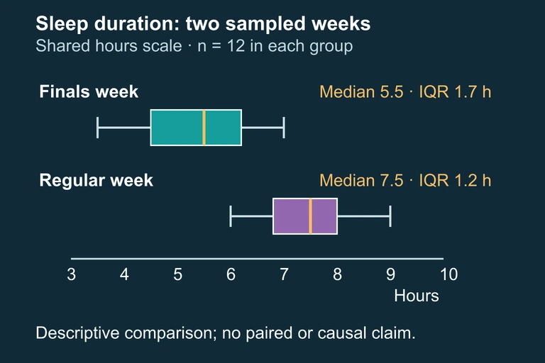Independent-group boxplots on a common scale, each with n=12. Medians are 5.5 and 7.5; interquartile ranges are 1.7 and 1.2. The sampled finals-week group has a lower median and a larger IQR than the regular-week group; summaries do not establish causation or full shape.

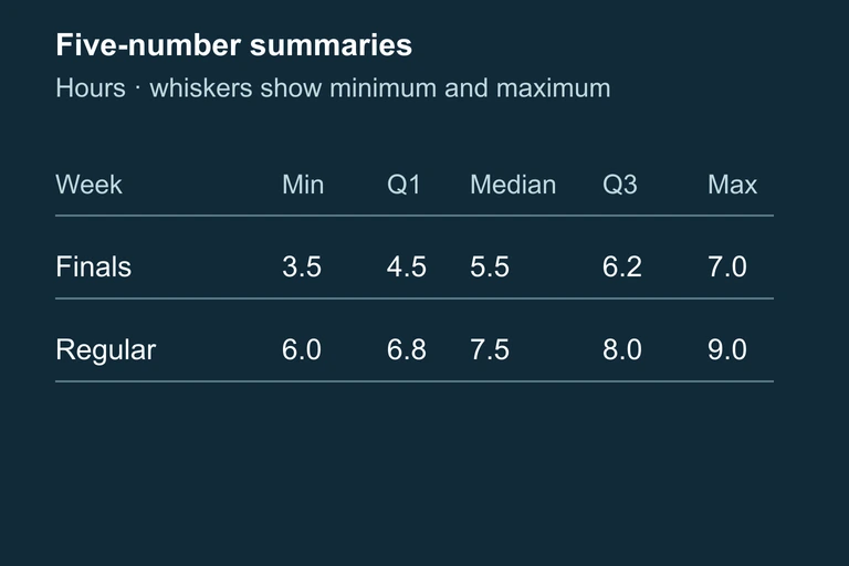Table of both groups’ five-number summaries. Boxplot whiskers represent minimum and maximum values.

SECTION 7

Common Strengths & Pitfalls

Even students who understand the SOCS framework often lose points on AP free-response questions because of avoidable errors. The table below contrasts effective comparison strategies with common mistakes, drawn from released AP scoring guidelines.

Effective Strategy ✓	Common Pitfall ✗
Use explicit comparative language: "Group A's median is higher than Group B's."	Describe each group in isolation without connecting them: "Group A's median is 72. Group B's median is 65."
Address all four SOCS features (shape, outliers, center, spread).	Mention only center, ignoring shape and/or spread.
Include specific numerical evidence: "The IQR for finals week (1.7 hrs) exceeds that of the regular week (1.2 hrs)."	Make vague claims: "One group is more spread out."
Use consistent statistics: if one distribution is skewed, report median and IQR for both.	Mix statistics: report the mean for one group and the median for the other.
Provide context: relate your comparison to the variable and groups being studied.	Write a generic comparison with no reference to the variables or real-world meaning.

Scoring strategies vs. common errors on AP distribution comparison questions

✦

THE COMPARISON PRINCIPLE

Think of each SOCS feature as a dimension. Describing one group's center without comparing it to the other group's center is like reporting only the latitude of a city and expecting someone to know where it is—you need both coordinates. Every feature you describe for one group must be explicitly compared to the same feature in the other group, with numerical support and context.

SECTION 8

Connection to Inference

Descriptive comparison of distributions is the essential first step, but it does not by itself establish whether observed differences are statistically significant. Later in the AP Statistics curriculum, you will encounter inferential methods—particularly the two-sample t-test and the two-sample t-interval—that allow you to determine whether a difference in means could plausibly be due to chance alone. Understanding how to compare distributions descriptively prepares you for those procedures in two critical ways: (1) checking conditions such as approximate normality or identifying outliers that might violate assumptions, and (2) developing intuition about whether a difference in centers is large relative to the spread within each group.

Descriptive Comparison (Unit 1)	Inferential Comparison (Units 7–8)
Describes the observed data	Generalizes from sample data to populations
Uses graphs and summary statistics (SOCS)	Uses test statistics, p-values, and confidence intervals
Answers: "How do these samples differ?"	Answers: "Is the difference likely real, or due to chance?"
No assumptions about random sampling required	Requires random sampling/assignment and normality conditions
Checks shape and outliers to choose appropriate statistics	Checks shape and outliers to verify inference conditions

Descriptive vs. inferential comparison of distributions

A useful heuristic: if the boxplots for two groups show substantial overlap (the boxes themselves are at similar positions on the axis), then a formal test may reveal no statistically significant difference. Conversely, if the boxes barely overlap or are entirely separated, there is strong visual evidence that the population centers differ. While this heuristic is not a substitute for a formal test, it builds the kind of statistical intuition that will serve you throughout the course and in professional data analysis.

SECTION 9

Practice Problems

Question 1: CONCEPTUAL

When comparing the distributions of test scores for two classes using side-by-side boxplots, a student writes: "The median for Class A is 78 and the median for Class B is 72. The IQR for Class A is 15 and the IQR for Class B is 10." Which of the following best describes what is missing from this comparison for a complete SOCS response?

A. The student needs to include a hypothesis test for the difference in medians.
B. The student needs to describe shape and outliers, use comparative language, and provide context.
C. The student needs to report the mean and standard deviation instead of the median and IQR.
D. The student needs to include a calculation of the coefficient of variation for each group.
E. The comparison is already complete; no additional information is needed.

Show answer (B)

B is correct. A complete SOCS comparison requires four elements: Shape, Outliers, Center, and Spread—all stated with comparative language and in context. The student addressed center and spread numerically but listed them in isolation ("median for A is 78" and "median for B is 72") without explicit comparative words like "higher than" or "greater than." Shape and outliers are entirely missing. A is incorrect because hypothesis testing is inferential, not part of a descriptive comparison. C is incorrect because median and IQR are perfectly appropriate (and preferred for skewed data). D is incorrect because the coefficient of variation is not part of the AP Statistics SOCS framework. E is incorrect because two of the four SOCS elements are missing and comparative language is absent.

Question 2: BASIC CALCULATION

A dataset for Group X has Q₁ = 20, median = 28, and Q₃ = 36. A dataset for Group Y has Q₁ = 25, median = 30, and Q₃ = 35. Which of the following statements correctly compares the spread of the middle 50% of these two groups?

A. Group X has greater spread (IQR = 16) than Group Y (IQR = 10).
B. Group Y has greater spread (IQR = 10) than Group X (IQR = 8).
C. Both groups have the same spread because their medians are only 2 apart.
D. Group Y has greater spread (IQR = 15) than Group X (IQR = 12).
E. The spread cannot be compared without knowing the standard deviations.

Show answer (A)

A is correct. The IQR is calculated as Q₃ − Q₁. For Group X: IQR = 36 − 20 = 16. For Group Y: IQR = 35 − 25 = 10. Since 16 > 10, the middle 50% of Group X's data is more spread out. B is incorrect because it miscalculates Group X's IQR as 8 (perhaps confusing Q₃ − median with Q₃ − Q₁). C is incorrect because the difference in medians measures center, not spread. D uses incorrect IQR calculations. E is incorrect because the IQR is a valid and commonly used measure of spread that does not require the standard deviation.

Question 3: INTERMEDIATE

Side-by-side boxplots show the distribution of commute times (in minutes) for employees at two offices. Office A's boxplot has its median line at 25 minutes, and the box extends from 18 to 35, with whiskers from 10 to 50 and one outlier plotted at 65. Office B's boxplot has its median line at 32 minutes, and the box extends from 27 to 40, with whiskers from 20 to 52 and no outliers. Which of the following is the best comparative statement?

A. Office A has a higher center and more spread than Office B.
B. Office B has a higher center than Office A, while Office A has a larger IQR and an outlier at 65 minutes.
C. Office A and Office B have similar distributions because their ranges are close (40 vs. 32 minutes).
D. Office A is symmetric while Office B is right-skewed, and both have the same variability.
E. Office B has a higher center and more spread than Office A, and Office A has an outlier.

Show answer (B)

B is correct. Office B's median (32) is higher than Office A's median (25), so Office B has a higher center. Office A's IQR = 35 − 18 = 17, while Office B's IQR = 40 − 27 = 13, so Office A has greater spread in the middle 50%. Office A also has an outlier at 65 minutes. A is incorrect because Office A has a lower center, not higher. C is incorrect because similar ranges do not mean similar distributions—center, shape, and IQR all differ. D is incorrect because boxplots alone cannot definitively determine symmetry vs. skew, and the variability differs. E correctly identifies Office B's higher center and the outlier, but incorrectly claims Office B has more spread—Office A's IQR (17) exceeds Office B's (13).

Question 4: APPLIED

4 pts

A nutritionist recorded the daily calorie intake for two groups of adults: 15 individuals following a Mediterranean diet and 15 individuals following a typical Western diet. The five-number summaries are shown below. Mediterranean diet: Min = 1450, Q₁ = 1650, Median = 1820, Q₃ = 1950, Max = 2100 Western diet: Min = 1600, Q₁ = 2050, Median = 2350, Q₃ = 2700, Max = 3400 The mean and standard deviation for the Mediterranean diet group are 1810 and 185, respectively. For the Western diet group, the mean and standard deviation are 2380 and 480. (a) Construct a complete comparison of the two distributions using the SOCS framework. Use comparative language and reference specific numerical values. (b) A colleague suggests reporting the mean and standard deviation for both groups. Explain whether this is appropriate given the information provided.

Show answer

Scoring Rubric (4 points): Part (a) — 3 points: Point 1 (Shape comparison): The Mediterranean diet distribution appears roughly symmetric (mean ≈ median: 1810 ≈ 1820), while the Western diet distribution appears right-skewed (mean = 2380 > median = 2350, and the distance from Q₃ to Max (700) greatly exceeds Q₁ to Min (450)), suggesting some individuals consume notably high calories. Point 2 (Center comparison with comparative language): The Western diet group has a substantially higher center than the Mediterranean diet group. The median calorie intake for the Western group (2350 calories) exceeds that of the Mediterranean group (1820 calories) by 530 calories. Point 3 (Spread comparison with comparative language and outlier check): The Western diet group is much more variable than the Mediterranean group. The IQR for the Western group (2700 − 2050 = 650 calories) is more than double the IQR for the Mediterranean group (1950 − 1650 = 300 calories), approximately 2.2 times as large. Using the 1.5 × IQR rule: For the Western group, the upper fence is 2700 + 1.5(650) = 3675, and the max (3400) falls within this fence, so there are no outliers. For the Mediterranean group, fences are 1650 − 450 = 1200 and 1950 + 450 = 2400; no outliers. Neither distribution has outliers. Part (b) — 1 point: Point 4: Because the Western diet distribution appears right-skewed, the median and IQR would be more appropriate resistant measures for that group. However, since the Mediterranean distribution is roughly symmetric, mean/standard deviation would work for that group. To ensure a consistent and fair comparison, the nutritionist should report median and IQR for both groups rather than mixing statistical pairs. If the colleague insists on using mean and standard deviation, it is important to note that the mean will overestimate the typical calorie intake for the right-skewed Western diet group.

Question 5: CRITICAL THINKING

4 pts

Two AP Statistics classes take the same exam. Class 1 (n = 30) has a mean score of 74 with a standard deviation of 8, and the distribution is approximately symmetric. Class 2 (n = 30) has a mean score of 74 with a standard deviation of 18, and the distribution is approximately symmetric. (a) Both classes have the same mean. Explain what the difference in standard deviations tells us about how students performed differently in the two classes. (b) Suppose a student scored 82 on the exam. Describe and compare this student's relative standing in each class. Use standardized scores (z-scores) to support your answer. (c) A school administrator says, "Both classes did equally well because they have the same average." Write a response explaining why this conclusion is incomplete and what additional information the comparison of distributions reveals.

Show answer

Scoring Rubric (4 points): Point 1 — Part (a), interpreting the difference in spread: The standard deviation of Class 2 (s = 18) is more than twice that of Class 1 (s = 8), meaning scores in Class 2 are far more spread out around the mean. In Class 1, students performed relatively consistently — most scores cluster within about 8 points of 74, roughly in the range 66 to 82. In Class 2, the typical deviation from the mean is 18 points, so scores range widely from roughly 56 to 92. Class 2 likely contains students who scored very high alongside students who scored very low, whereas Class 1's students performed more uniformly. Point 2 — Part (b), z-score calculations and comparison: In Class 1: z = (82 − 74) / 8 = 8 / 8 = 1.00. In Class 2: z = (82 − 74) / 18 = 8 / 18 ≈ 0.44. A score of 82 places the student one full standard deviation above the mean in Class 1, which is a relatively high position. In Class 2, the same score is only about 0.44 standard deviations above the mean, a much less distinguished position. Therefore, a score of 82 represents a stronger relative performance in Class 1 than in Class 2. Point 3 — Part (b), connecting z-scores to relative standing: Because both distributions are approximately symmetric, we can interpret the z-scores in terms of percentile position. A z-score of 1.00 in Class 1 places the student at approximately the 84th percentile, meaning the student scored higher than roughly 84% of classmates. A z-score of 0.44 in Class 2 places the student at approximately the 67th percentile. Even though the raw score is the same, the student's relative standing is notably higher in Class 1, where the smaller spread means fewer students scored as high. Point 4 — Part (c), explaining why center alone is insufficient: The administrator's conclusion is incomplete because comparing distributions requires examining spread, shape, and potential outliers in addition to center. Two distributions can have identical means yet tell very different stories about student performance. Class 2's much larger standard deviation indicates a wider gap between the highest and lowest performers, which could signal disparities in preparation, engagement, or instructional effectiveness. A complete comparison would note that while the centers are the same, the variability in Class 2 is substantially greater, meaning the two classes did not perform "equally well" in any holistic sense. Consistent performance near the mean (Class 1) is qualitatively different from highly variable performance around the same mean (Class 2).

SUMMARY

Lesson Summary

Summary

Comparing distributions of a quantitative variable requires a systematic examination of four features, remembered by the acronym SOCS: Shape, Outliers, Center, and Spread. Every comparison must use explicit comparative language ("higher than," "more variable than," "whereas") rather than isolated descriptions of each group. Use side-by-side boxplots, parallel dotplots, or back-to-back stemplots on a shared axis for visual comparison, and support your observations with specific numerical evidence (medians, IQRs, means, standard deviations).

Choose your summary statistics to match the shape of the distributions: use median and IQR for skewed distributions and mean and standard deviation for symmetric distributions, and always use the same pair of statistics for both groups. Remember that this descriptive comparison lays the groundwork for later inferential procedures (two-sample t-tests and confidence intervals) that will let you determine whether observed differences are statistically significant.