Combining Random Variables - AP Statistics

SECTION 1

Historical Context & Motivation

Virtually every real-world measurement is the result of combining several sources of variability. When an insurance company estimates total claims, it sums thousands of individual policyholder losses; when a manufacturer checks whether two parts will fit together, it examines the difference in their dimensions. The mathematics of combining random variables provides the rules that make such analyses tractable. Without these rules, extending probability theory beyond single-variable problems would be nearly impossible.

1718 • De Moivre's Doctrine of Chances

Abraham de Moivre published foundational work on sums of independent outcomes in games of chance, laying groundwork for additive variance rules.

1812 • Laplace's Théorie Analytique

Pierre-Simon Laplace formalized the idea that the distribution of a sum of independent variables is the convolution of their individual distributions, generalizing earlier gambling-based results.

1900 • Pearson & Biometrics

Karl Pearson applied linear combination rules to biological measurements, demonstrating that variance components could be isolated and summed in hereditary studies.

1933 • Kolmogorov's Axioms

Andrey Kolmogorov placed probability on rigorous measure-theoretic foundations, providing the formal justification for expectation linearity and the variance addition rule for independent variables.

The central question these developments addressed is deceptively simple: if you know the mean and variance of two separate random variables, what can you say about the mean and variance of their sum or difference? The answer—codified in the rules we study in this lesson—turns out to be elegant, powerful, and occasionally counterintuitive, especially the fact that variances add even when you subtract random variables.

SECTION 2

Core Principles & Definitions

Before diving into formulas, it is essential to internalize several foundational ideas. These principles govern every calculation you will perform when combining random variables, and a clear grasp of them will prevent the most common AP exam errors.

Linearity of Expectation

The expected value of a sum (or difference) equals the sum (or difference) of the expected values. This holds always—regardless of whether the variables are independent.

Variance Addition Rule

When two random variables are independent, the variance of their sum or difference equals the sum of their individual variances. Variances always add—never subtract.

Independence Requirement

The variance addition rule requires independence. If two variables are correlated, a covariance term must be included. On the AP exam, problems typically state or imply independence.

Linear Transformations

Multiplying a random variable by a constant a multiplies the mean by a and multiplies the variance by a². Adding a constant shifts the mean but does not change the variance.

Standard Deviation from Variance

You cannot add standard deviations directly. Always work in variance, combine variances, then take the square root at the end to obtain the combined standard deviation.

SECTION 3

Visualizing Combined Distributions

The diagram below illustrates how two independent normal random variables combine. Variable X has mean 50 and standard deviation 4, while variable Y has mean 30 and standard deviation 3. Notice that the combined distribution X + Y is centered at 80 (the sum of the means) and is wider than either individual distribution because the variances add, giving a standard deviation of 5.

The cyan curve represents X (μ = 50, σ = 4), the violet curve represents Y (μ = 30, σ = 3), and the emerald curve shows X + Y (μ = 80, σ = 5). The combined curve is wider because the variances add: 4² + 3² = 25, so the combined standard deviation is √25 = 5.

A critical observation from this diagram is that the combined distribution is always wider than either individual distribution. This holds true whether we compute X + Y or X − Y. In the subtraction case, the center would shift to 50 − 30 = 20, but the spread would remain σ = 5. The width of the combined distribution reflects the total uncertainty contributed by both variables, and uncertainty cannot cancel through subtraction of independent quantities.

SECTION 4

Mathematical Framework

The rules for combining random variables fall into two categories: linear transformations of a single variable (shifting and scaling) and linear combinations of two or more variables. Both sets of rules are testable on the AP exam, and fluency with the notation below is essential.

Linear Transformation: Y = a + bX

MEAN OF A LINEAR TRANSFORMATION

μ(a + bX) = a + b · μ_X

Adding a constant a shifts the center; multiplying by b scales the center.

VARIANCE OF A LINEAR TRANSFORMATION

σ²(a + bX) = b² · σ²_X

The additive constant a has no effect on spread. The multiplier b is squared when applied to variance, so σ(a + bX) = |b| · σ_X.

Combining Two Independent Variables: X ± Y

MEAN OF A SUM OR DIFFERENCE

μ(X ± Y) = μ_X ± μ_Y

Means follow the operation sign. This rule holds whether or not X and Y are independent.

VARIANCE OF A SUM OR DIFFERENCE (INDEPENDENT)

σ²(X ± Y) = σ²_X + σ²_Y

Variances always add when X and Y are independent—the plus sign applies regardless of whether the variables are added or subtracted. This is the most commonly tested rule on the AP exam.

ℹ

Common Pitfall

SECTION 5

Key Scenarios & Classifications

On the AP exam, combining random variables appears in several distinct forms. Recognizing which scenario is at play determines which formula to use. The diagram below classifies the most common situations and shows the relevant formulas for each.

Decision flowchart for combining random variables. Start at the top and follow the branches. Note the special case at the bottom: doubling a single variable (2X) uses the linear transformation rule, not the sum rule.

The 2X vs. X₁ + X₂ Distinction

This is one of the most commonly tested distinctions on the AP exam. Suppose X has mean 10 and standard deviation 3. If you double the single variable, you get 2X, which has mean 20 and standard deviation 2 × 3 = 6 (variance = 4 × 9 = 36). But if X₁ and X₂ are two independent observations from the same distribution, then X₁ + X₂ has mean 20 but standard deviation √(9 + 9) = √18 ≈ 4.24 (variance = 18). The means are identical, but the variances differ because 2X amplifies a single source of randomness while X₁ + X₂ draws from two independent sources.

Quantity	Mean	Variance	Std Dev
X	10	9	3
2X (linear transformation)	20	36	6
X₁ + X₂ (independent copies)	20	18	≈ 4.24

Comparison of 2X versus X₁ + X₂ when μ_X = 10 and σ_X = 3

A filling line loads bottles into trays while one statistic is recorded for each tray. A production line can combine two independent measurements or scale one measurement. Those operations can share a mean while producing different variances.

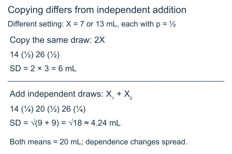Two outcome distributions contrast doubling the same 7-or-13 draw with adding two independent draws. Suppose X is equally likely to be 7 or 13. Then 2X is 14 or 26 and has standard deviation 6. For independent X₁ and X₂, their sum is 14, 20 or 26 with probabilities 1/4, 1/2 and 1/4 and standard deviation √18. Both means are 20.

SECTION 6

Worked Example

A coffee shop sells lattes and pastries. Let L represent the profit on a randomly selected latte with μ_L = $2.50 and σ_L = $0.40, and let P represent the profit on a randomly selected pastry with μ_P = $1.80 and σ_P = $0.30. Assume L and P are independent. Find the mean and standard deviation of the total profit T = L + P on one latte-and-pastry combo, and the mean and standard deviation of the difference D = L − P.

Worked example

1
Step 1 — Identify Given Values

μ_L = 2.50, σ_L = 0.40, μ_P = 1.80, σ_P = 0.30. The variables L and P are independent.
2
Step 2 — Find the Mean of the Sum

By linearity of expectation: μ_T = μ_L + μ_P = 2.50 + 1.80

μ_T = $4.30
3
Step 3 — Find the Variance of the Sum

Since L and P are independent: σ²_T = σ²_L + σ²_P = (0.40)² + (0.30)² = 0.16 + 0.09

σ²_T = 0.25
4
Step 4 — Find the Standard Deviation

σ_T = √0.25 = 0.50

σ_T = $0.50

Worked example

1
Step 1 — Find the Mean of the Difference

μ_D = μ_L − μ_P = 2.50 − 1.80

μ_D = $0.70
2
Step 2 — Find the Variance of the Difference

Even though we are subtracting, variances still add: σ²_D = σ²_L + σ²_P = 0.16 + 0.09

σ²_D = 0.25
3
Step 3 — Standard Deviation of the Difference

σ_D = √0.25 = 0.50. Notice this is the same standard deviation as the sum—confirming that variance addition is unaffected by the sign of the combination.

σ_D = $0.50

SECTION 7

Common Mistakes & Comparisons

Mastering the mechanics of combining random variables is only half the battle. On the AP exam, many points are lost to avoidable conceptual errors. The table below catalogues the most frequent mistakes alongside the correct reasoning.

Common Mistake	Why It's Wrong	Correct Approach
Adding standard deviations: σ(X + Y) = σ_X + σ_Y	Standard deviations don't add linearly. Only variances add for independent variables.	σ(X + Y) = √(σ²_X + σ²_Y)
Subtracting variances: σ²(X − Y) = σ²_X − σ²_Y	Subtraction increases total uncertainty. Variance cannot be negative, and independent errors compound.	σ²(X − Y) = σ²_X + σ²_Y
Confusing 2X with X₁ + X₂	2X scales one observation; X₁ + X₂ sums two independent observations. They yield different variances.	Var(2X) = 4σ²_X; Var(X₁ + X₂) = 2σ²_X
Applying variance rule to dependent variables	The simple addition rule requires independence. Dependent variables introduce a covariance term.	Verify independence is stated or implied before using σ²_X + σ²_Y.
Forgetting to square the constant in transformations	Var(3X) = 9σ²_X, not 3σ²_X. The constant must be squared.	Var(bX) = b²·Var(X)

Five most common errors when combining random variables

★

Key takeaway

EXAM STRATEGY

SECTION 8

Connections to Advanced Topics

The rules for combining random variables serve as the mathematical backbone for several major topics you will encounter later in the AP Statistics course and in college-level probability and inference. Understanding these connections reveals why mastering the present topic is so important.

This Lesson	Where It Leads
μ(X₁ + X₂ + … + Xₙ) = nμ	Leads directly to the expected value of the sampling distribution of the sample mean: E(X̄) = μ.
Var(X₁ + … + Xₙ) = nσ²	After dividing by n², gives Var(X̄) = σ²/n — the foundation of the Central Limit Theorem.
σ²(X − Y) = σ²_X + σ²_Y	Underpins the two-sample t-test for the difference of means and the standard error formula for p̂₁ − p̂₂.
Linear transformation rules	Used in standardizing variables to z-scores: Z = (X − μ)/σ is a linear transformation with a = −μ/σ, b = 1/σ.

How combining-random-variable rules connect to later AP Statistics topics

Beyond AP Statistics, the general version of the variance-of-a-sum formula for dependent variables includes the covariance: Var(X + Y) = Var(X) + Var(Y) + 2Cov(X, Y). When X and Y are independent, Cov(X, Y) = 0, which collapses to the simpler rule studied here. In multivariate statistics and portfolio theory, the covariance matrix generalizes these ideas to arbitrarily many correlated variables, enabling analysts to quantify risk in financial portfolios and measurement systems. The independence assumption you are learning now is thus a special—but extremely common and practically useful—case of a much broader framework.

SECTION 9

Practice Problems

Question 1: CONCEPTUAL

Random variables X and Y are independent. Which of the following statements is true about the standard deviation of X − Y? (A) σ(X − Y) = σ_X − σ_Y (B) σ(X − Y) = σ_X + σ_Y (C) σ(X − Y) = √(σ²_X + σ²_Y) (D) σ(X − Y) = √(σ²_X − σ²_Y) (E) σ(X − Y) = σ²_X + σ²_Y

A. σ(X − Y) = σ_X − σ_Y
B. σ(X − Y) = σ_X + σ_Y
C. σ(X − Y) = √(σ²_X + σ²_Y)
D. σ(X − Y) = √(σ²_X − σ²_Y)
E. σ(X − Y) = σ²_X + σ²_Y

Show answer (C)

The correct answer is (C). For independent random variables, variances always add regardless of whether the variables are added or subtracted: σ²(X − Y) = σ²_X + σ²_Y. Taking the square root gives σ(X − Y) = √(σ²_X + σ²_Y). Choice (A) is wrong because standard deviations do not subtract; uncertainty increases when combining independent variables. Choice (B) incorrectly adds standard deviations rather than taking the square root of summed variances. Choice (D) incorrectly subtracts variances—variance can never decrease through combining independent variables. Choice (E) gives the variance, not the standard deviation, since it omits the square root.

Question 2: BASIC CALCULATION

Let X be a random variable with μ_X = 12 and σ_X = 5. A new variable is defined as Y = 3X + 7. What are the mean and standard deviation of Y? (A) μ_Y = 43, σ_Y = 22 (B) μ_Y = 43, σ_Y = 15 (C) μ_Y = 43, σ_Y = 75 (D) μ_Y = 36, σ_Y = 15 (E) μ_Y = 43, σ_Y = 225

A. μ_Y = 43, σ_Y = 22
B. μ_Y = 43, σ_Y = 15
C. μ_Y = 43, σ_Y = 75
D. μ_Y = 36, σ_Y = 15
E. μ_Y = 43, σ_Y = 225

Show answer (B)

The correct answer is (B). Using the linear transformation rules: μ_Y = 3(12) + 7 = 36 + 7 = 43, and σ_Y = |3| × σ_X = 3 × 5 = 15. Choice (A) is wrong because 22 does not correspond to any valid calculation. Choice (C) gives 75, which equals b² × σ_X = 9 × 5 × (something)—it actually equals 3σ²_X, mixing up variance and standard deviation. Choice (D) uses 36 for the mean, forgetting to add the constant 7. Choice (E) gives σ_Y = 225 = (3)² × (5)² = the variance, not the standard deviation.

Question 3: INTERMEDIATE

A random variable X has mean 20 and standard deviation 6. If X₁ and X₂ are independent observations from this distribution, which of the following correctly compares Var(2X₁) and Var(X₁ + X₂)? (A) Var(2X₁) = Var(X₁ + X₂) = 72 (B) Var(2X₁) = 144; Var(X₁ + X₂) = 72 (C) Var(2X₁) = 72; Var(X₁ + X₂) = 144 (D) Var(2X₁) = Var(X₁ + X₂) = 144 (E) Var(2X₁) = 144; Var(X₁ + X₂) = 36

A. Var(2X₁) = Var(X₁ + X₂) = 72
B. Var(2X₁) = 144; Var(X₁ + X₂) = 72
C. Var(2X₁) = 72; Var(X₁ + X₂) = 144
D. Var(2X₁) = Var(X₁ + X₂) = 144
E. Var(2X₁) = 144; Var(X₁ + X₂) = 36

Show answer (B)

The correct answer is (B). Var(X) = 36. For the linear transformation 2X₁: Var(2X₁) = 2² × 36 = 144. For two independent observations: Var(X₁ + X₂) = 36 + 36 = 72. Choice (A) incorrectly assigns 72 to both. Choice (C) reverses the two values. Choice (D) assigns 144 to both, wrongly treating the sum of independent copies as equivalent to doubling one observation. Choice (E) uses 36 for the sum, as though adding zero variance.

Question 4: APPLIED

A manufacturing process produces bolts with mean diameter μ_B = 10.00 mm and standard deviation σ_B = 0.05 mm, and nuts with mean inner diameter μ_N = 10.20 mm and standard deviation σ_N = 0.04 mm. Bolt and nut diameters are independent. An engineer defines the clearance as C = N − B (nut inner diameter minus bolt diameter). A bolt-nut pair is considered acceptable if the clearance is between 0.10 mm and 0.30 mm. (a) Find the mean and standard deviation of C. (b) Assuming C is approximately normal, find the probability that a randomly selected bolt-nut pair is acceptable. (c) A redesign reduces σ_B to 0.03 mm. Without recalculating the exact probability, explain how this change affects the distribution of C and the proportion of acceptable pairs.

Show answer

(a) [2 points] μ_C = μ_N − μ_B = 10.20 − 10.00 = 0.20 mm. Since B and N are independent, σ²_C = σ²_N + σ²_B = (0.04)² + (0.05)² = 0.0016 + 0.0025 = 0.0041. Thus σ_C = √0.0041 ≈ 0.0640 mm. (b) [2 points] Use σ_C = √0.0041 ≈ 0.064031242 mm without premature rounding. Then z_low = −0.1/√0.0041 ≈ −1.561737619 and z_high ≈ 1.561737619. Thus P(0.10 < C < 0.30) = 2Φ(1.561737619) − 1 ≈ 0.881650. About 88.2% of pairs are acceptable under the approximate normal model. (c) [2 points] Reducing σ_B decreases the total variance of C. The new σ²_C = (0.04)² + (0.03)² = 0.0025, giving σ_C = 0.05 mm. Since the mean clearance remains 0.20 mm (the center of the acceptable range), a narrower distribution concentrates more area within the acceptable interval, increasing the proportion of acceptable pairs. Normal clearance model centered at 0.20 mm with standard deviation √(0.04²+0.05²) mm. The shaded acceptable interval 0.10 to 0.30 mm has probability about 88.2%.

Normal clearance model centered at 0.20 mm with standard deviation √(0.04²+0.05²) mm. The shaded acceptable interval 0.10 to 0.30 mm has probability about 88.2%.

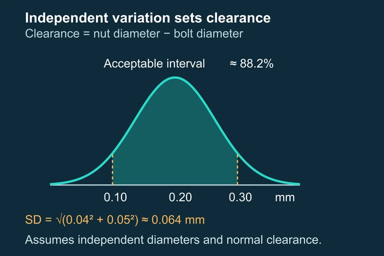Independent nut and bolt variation combine through added variances for their clearance, under the stated distribution assumptions.

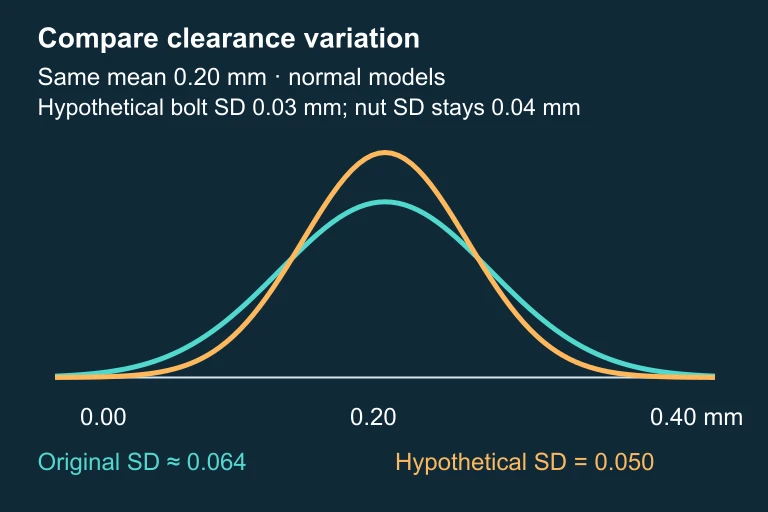Two normal clearance models centered at 0.20 mm, with standard deviations about 0.064 and 0.050 mm. The narrower model has a taller density and more probability in the acceptance interval.

Question 5: CRITICAL THINKING

A student claims: 'If X and Y are independent random variables each with variance 100, then the variance of their average, (X + Y)/2, equals 100 because averaging should not change the variance.' Evaluate this claim. (a) Compute Var((X + Y)/2) and show that the student's claim is incorrect. (b) Generalize: if X₁, X₂, …, Xₙ are independent with common variance σ², derive a formula for Var(X̄) where X̄ = (X₁ + X₂ + … + Xₙ)/n. (c) Explain conceptually why averaging reduces variance and connect this result to inference in AP Statistics.

Show answer

(a) [2 points] Let S = X + Y. Since X and Y are independent, Var(S) = Var(X) + Var(Y) = 100 + 100 = 200. Now (X + Y)/2 = (1/2)S, which is a linear transformation with b = 1/2. So Var((X + Y)/2) = (1/2)² × 200 = (1/4)(200) = 50. The student's claim is incorrect; the variance is 50, not 100. (b) [2 points] Var(X₁ + X₂ + … + Xₙ) = nσ² by the variance addition rule for independent variables. Then X̄ = (1/n)(X₁ + … + Xₙ), so Var(X̄) = (1/n)² × nσ² = σ²/n. The variance of the sample mean equals the population variance divided by the sample size. (c) [2 points] Averaging reduces variance because individual deviations from the mean partially offset each other when combined—some observations fall above μ and others below, so their sum is less variable per observation than any single observation. This is the mathematical basis for the standard error formula σ/√n used throughout AP Statistics inference. It explains why larger samples produce more precise estimates: as n increases, Var(X̄) = σ²/n decreases, narrowing confidence intervals and increasing the power of hypothesis tests.