Setting Up a Chi-Square Test for Homogeneity or Independence - AP Statistics

SECTION 1

Historical Context & Motivation

Long before the formal apparatus of hypothesis testing existed, researchers confronted a deceptively simple question: when observed counts in a table of categorical data deviate from what we would expect under some null model, how do we decide whether those deviations are large enough to matter? The answer required a test statistic whose sampling distribution was known, and the development of that statistic — the chi-square (χ²) statistic — reshaped how scientists analyze categorical data. Understanding the historical trajectory of this tool illuminates why the setup of a chi-square test matters just as much as the computation itself.

1900 • Pearson's Chi-Square Test

Karl Pearson published his seminal paper introducing the χ² goodness-of-fit test, providing the first rigorous method for comparing observed categorical frequencies to expected frequencies under a theoretical model.

1922 • Fisher's Refinement

R. A. Fisher clarified the correct degrees of freedom for contingency tables and formalized the distinction between testing a model's fit and testing for association between two categorical variables.

1930s • Homogeneity vs. Independence

Statisticians recognized that the same χ² computational machinery could serve two distinct research designs — comparing distributions across populations (homogeneity) or assessing association within a single population (independence).

1950s–70s • Textbook Codification

Introductory statistics textbooks formalized the conditions, hypotheses, and step-by-step procedures students use today, establishing the 'state–plan–do–conclude' framework for inference with categorical data.

Despite the shared computation, the test for homogeneity and the test for independence begin with fundamentally different research designs and hypotheses. The AP Statistics exam rewards students who can clearly articulate which test applies to a given scenario, state the correct hypotheses, verify the conditions, and interpret results in context. This lesson addresses the critical question: how do you set up each test correctly before any arithmetic begins?

SECTION 2

Core Principles & Definitions

Before you can set up a chi-square test correctly, you need a firm grasp of several interrelated concepts. Both the test for homogeneity and the test for independence analyze data organized in a two-way table (also called a contingency table), where one categorical variable defines the rows and another defines the columns. The cells contain observed counts — not percentages or proportions. The distinction between the two tests lies entirely in how the data were collected and what the null hypothesis claims.

Test for Homogeneity

Used when independent random samples are drawn from two or more distinct populations (or treatment groups), and the researcher asks whether the distribution of a single categorical variable is the same across all populations.

Test for Independence

Used when a single random sample is drawn from one population, and the researcher asks whether two categorical variables are associated (dependent) or independent within that population.

Expected Counts

Under the null hypothesis, the expected count for each cell is calculated as (row total × column total) / grand total. These values represent what we would observe if the null hypothesis were true.

Degrees of Freedom

For an r × c table, df = (r − 1)(c − 1). The degrees of freedom determine which chi-square distribution is used to compute the p-value.

Conditions for Inference

Both tests require: (1) data collected via random sampling or random assignment, (2) independent observations, and (3) all expected counts are at least 5. These conditions must be verified before computing the test statistic.

✦

KEY TAKEAWAY

Think of the distinction like this: a test for homogeneity is like a quality-control engineer sampling widgets from three different factories and asking whether the defect-rate distribution is the same at each factory — multiple populations, one variable. A test for independence is like a market researcher surveying one city's residents and asking whether brand preference is associated with age group — one population, two variables. The arithmetic is identical, but the story behind the data determines which test you name.

SECTION 3

Visual Explanation: Study Design Decision Flowchart

One of the most common exam pitfalls is misidentifying which chi-square test to use. The following flowchart walks you through the decision process based entirely on how the data were collected. Start at the top and follow the arrows to determine the correct test setup.

The decision hinges on the sampling design: if separate random samples come from distinct populations (or treatment groups), use a test for homogeneity. If a single sample is classified on two categorical variables, use a test for independence. The formula and degrees of freedom are identical in both cases.

Notice that the flowchart converges at the bottom: both tests use the same χ² formula and the same degrees of freedom. The only differences are (1) the research design, (2) the wording of the hypotheses, and (3) which totals in the two-way table are predetermined by the design. On the AP exam, identifying these distinctions in context is worth significant credit in free-response scoring.

A university campus provides a setting for comparing sampling and study-design routes. The way people or groups enter a study determines its design. Sampling within groups, selecting whole groups and assigning treatments answer different questions.

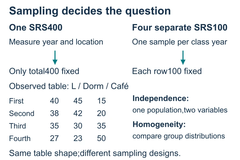A four-by-three observed table with row totals 100 and column totals 140, 140 and 120 is linked to independence and homogeneity designs. For the displayed 400-student table, expected counts in each row are 35, 35 and 30, and df = (4 − 1)(3 − 1) = 6. One random sample classified twice tests independence; separately sampled class-year groups test homogeneity.

SECTION 4

Mathematical Framework

Setting up the chi-square test requires computing expected counts under the null hypothesis and then measuring how far the observed data depart from those expectations. The mathematical machinery is compact but conceptually powerful: every cell in the two-way table contributes a term to the test statistic, and the sum of those terms follows a known distribution (under certain conditions) that lets us compute a p-value.

EXPECTED COUNT

E = (row total × column total) / grand total

For each cell in the two-way table, E represents the count we would expect if the null hypothesis were true. This formula works identically for both the homogeneity and independence tests.

CHI-SQUARE TEST STATISTIC

χ² = Σ (O − E)² / E

O = observed count in a cell, E = expected count in that cell. The sum is taken over all cells in the table. Large values of χ² provide evidence against H₀.

DEGREES OF FREEDOM

df = (r − 1)(c − 1)

r = number of rows, c = number of columns. The degrees of freedom determine the shape of the χ² distribution used to find the p-value. For a 3 × 4 table, df = (3 − 1)(4 − 1) = 6.

Stating the Hypotheses

Although the computation is identical, the hypotheses must match the study design. For a test for homogeneity: H₀ states that the distribution of the categorical response variable is the same for all populations (or treatment groups); Hₐ states that at least one population's distribution differs. For a test for independence: H₀ states that the two categorical variables are independent in the population; Hₐ states that the two variables are not independent (i.e., they are associated). On the AP exam, you must state these hypotheses in the context of the given problem, not just symbolically.

💡

Exam Tip

The chi-square test is always one-sided in the upper tail: large values of χ² provide evidence against H₀. You never write a two-sided alternative or look at a lower tail for this test. All p-values come from P(χ² ≥ observed value).

SECTION 5

Checking the Conditions for Inference

Before computing the χ² statistic, you must verify three conditions. On the AP exam, failing to check conditions — or checking them incorrectly — is a common source of lost points on free-response questions. The conditions are the same for both the homogeneity and independence tests, though the way you describe the randomness condition differs slightly based on the study design.

All three conditions — Random, Independent, and Large Counts — must be verified before proceeding. The Large Counts condition checks expected counts, not observed counts. The way you verify the Random condition depends on whether the study involves multiple populations (homogeneity) or a single population (independence).

A critical detail that many students overlook: the Large Counts condition applies to expected counts, not observed counts. If even one expected count falls below 5, the χ² approximation to the true sampling distribution becomes unreliable, and the test should not be performed in its standard form. In practice, this means you must compute (or at least spot-check) expected counts before running the test — which is why setting up the test carefully is so important.

⚠

Common Mistake

Students sometimes write 'the sample size is large enough' without explicitly computing expected counts. On the AP exam, you must show that every expected count is at least 5. Stating the condition in general terms without verification earns no credit.

SECTION 6

Worked Example: Setting Up a Chi-Square Test

A university's admissions office surveyed a random sample of 400 current students and recorded each student's class year (Freshman, Sophomore, Junior, Senior) and preferred study location (Library, Dorm Room, Coffee Shop). The admissions office wants to know whether preferred study location is associated with class year. Here is the observed data:

	Library	Dorm Room	Coffee Shop	Row Total
Freshman	40	45	15	100
Sophomore	38	42	20	100
Junior	35	30	35	100
Senior	27	23	50	100
Col Total	140	140	120	400

Observed counts: Study location by class year (n = 400)

Setting Up the Chi-Square Test

1
Step 1 — Identify the Correct Test

A single random sample of 400 students was drawn from one population (current students at this university), and each student was classified on two categorical variables: class year and preferred study location. Because there is one sample and two categorical variables, this is a chi-square test for independence.

Test for Independence
2
Step 2 — State the Hypotheses

H₀: Class year and preferred study location are independent among students at this university. Hₐ: Class year and preferred study location are not independent (they are associated) among students at this university. Note that the hypotheses are stated in the context of the problem, not just as abstract symbols.

H₀: independence; Hₐ: association
3
Step 3 — Check the Random Condition

The problem states that the 400 students were a random sample of current students at this university. This satisfies the Random condition.

✓ Random sample stated
4
Step 4 — Check the 10% / Independence Condition

Since sampling was done without replacement, we need 400 ≤ 10% of all current students at this university. It is reasonable to assume the university has at least 4,000 students, so the 10% condition is satisfied and individual observations can be treated as independent.

✓ 400 ≤ 10% of population
5
Step 5 — Compute Expected Counts and Check Large Counts Condition

Expected count for each cell = (row total × column total) / 400. For Freshman–Library: (100 × 140) / 400 = 35. For Freshman–Dorm: (100 × 140) / 400 = 35. For Freshman–Coffee Shop: (100 × 120) / 400 = 30. Since all row totals are 100 and column totals are 140, 140, and 120, the expected counts for every row are 35, 35, and 30 respectively. All twelve expected counts are well above 5, so the Large Counts condition is satisfied.

✓ All expected counts ≥ 5 (minimum is 30)
6
Step 6 — State the Degrees of Freedom and Test Setup

The table has r = 4 rows and c = 3 columns, so df = (4 − 1)(3 − 1) = 3 × 2 = 6. We will use a χ² distribution with 6 degrees of freedom to compute the p-value. The test statistic is χ² = Σ (O − E)² / E, summed over all 12 cells. The test is now fully set up; computation of the test statistic and p-value would follow.

df = 6; χ² distribution with 6 df

SECTION 7

Comparing Homogeneity, Independence, and Goodness-of-Fit

Students often confuse the three chi-square tests because they all involve categorical data and similar-looking formulas. The table below organizes the key differences along the dimensions that matter most for setting up each test: the study design, the hypotheses, the type of table, and the degrees of freedom formula.

Feature	Goodness-of-Fit	Homogeneity	Independence
# of variables	1 categorical variable	1 categorical variable across ≥ 2 populations	2 categorical variables in 1 population
# of samples	1 sample	≥ 2 independent samples	1 sample
Table type	One-way (1 × c)	Two-way (r × c)	Two-way (r × c)
H₀	Distribution matches a specified model	Distribution is the same across all populations	The two variables are independent
Degrees of freedom	k − 1 (k = # categories)	(r − 1)(c − 1)	(r − 1)(c − 1)
Expected counts	np₀ for each category	(row total × col total) / n	(row total × col total) / n

Comparison of the three chi-square tests in AP Statistics

✦

KEY TAKEAWAY

The homogeneity and independence tests are computational twins — they share the same formula for expected counts, the same test statistic, and the same degrees of freedom. Think of them as two different experimental protocols that happen to produce the same type of data table. Just as a clinical trial (random assignment to treatments) and an observational cohort study (random sampling of existing groups) can both produce a 2 × 2 table of outcomes, the research design — not the table — determines which test you name and how you write your hypotheses.

SECTION 8

Connections to Advanced Theory

The chi-square tests you learn in AP Statistics are special cases of a broader inferential framework. Understanding where these tests sit in the larger landscape of statistics helps you appreciate both their power and their limitations, and it previews material you will encounter in college-level courses.

AP Statistics Level	Advanced / College Level
χ² test statistic: Σ (O − E)² / E	Derived as −2 × log-likelihood ratio (G-test), which is asymptotically equivalent to Pearson's χ²
Large counts condition: all E ≥ 5	When expected counts are small, Fisher's exact test or permutation-based methods provide exact p-values
Reject or fail to reject H₀	Standardized residuals (O − E) / √E identify which cells contribute most to the χ² statistic — a form of post-hoc analysis
Two-way tables only	Log-linear models extend χ² analysis to multi-way contingency tables with three or more categorical variables
No effect-size measure required	Cramér's V and the contingency coefficient quantify the strength of association, supplementing the significance test

AP-level chi-square concepts and their advanced extensions

For the AP exam, you do not need to know Fisher's exact test, log-linear models, or Cramér's V. However, understanding that the chi-square test is an approximation that improves with larger expected counts deepens your understanding of why the conditions matter. The requirement that all expected counts be at least 5 is a practical threshold below which the χ² distribution becomes a poor model for the true sampling distribution of the test statistic. In more advanced courses, you will learn exact and simulation-based alternatives that remove this restriction.

SECTION 9

Practice Problems

Question 1: CONCEPTUAL

A researcher randomly selects 200 adults from City A and 200 adults from City B and asks each person to classify their primary mode of transportation as Car, Public Transit, or Bicycle. Which chi-square test is appropriate for determining whether the distribution of transportation mode is the same in both cities?

A. Chi-square goodness-of-fit test
B. Chi-square test for independence
C. Chi-square test for homogeneity
D. Two-sample z-test for proportions
E. Matched-pairs t-test

Show answer (C)

The correct answer is C. Two independent random samples were drawn from two distinct populations (City A and City B), and the researcher asks whether the distribution of a single categorical variable (transportation mode) is the same across both. This is the definition of a test for homogeneity. A (goodness-of-fit) is wrong because it involves only one sample compared to a specified model, not two populations. B (independence) is wrong because there are two separate samples, not one sample classified on two variables. D (two-sample z-test) applies to comparing two proportions for a single binary outcome, not a three-category variable. E (matched-pairs t-test) applies to quantitative paired data, not categorical data.

Question 2: BASIC CALCULATION

In a 3 × 4 contingency table with a grand total of 600, one cell has a row total of 150 and a column total of 200. What is the expected count for that cell, and what are the degrees of freedom for the test?

A. E = 50; df = 6
B. E = 50; df = 11
C. E = 75; df = 6
D. E = 50; df = 12
E. E = 75; df = 11

Show answer (A)

The correct answer is A. The expected count is (row total × column total) / grand total = (150 × 200) / 600 = 30,000 / 600 = 50. Degrees of freedom = (r − 1)(c − 1) = (3 − 1)(4 − 1) = 2 × 3 = 6. B is wrong because df = 11 would arise from (r − 1) + (c − 1) = 2 + 3 = 5 or some other incorrect formula — the correct formula multiplies, not adds. C is wrong because 75 = 150 × 200 / 400, using the wrong grand total. D uses df = r × c = 12, which is the total number of cells, not degrees of freedom. E combines both errors from C and B.

Question 3: INTERMEDIATE

A health researcher randomly surveys 500 adults from a single metropolitan area and records each person's exercise frequency (None, Moderate, Vigorous) and self-reported health status (Poor, Fair, Good, Excellent). The researcher wishes to determine whether exercise frequency and health status are related. State the appropriate hypotheses and identify one expected count that must be checked. The table shows that 120 people exercise vigorously and 85 people report Poor health. What is the expected count for the Vigorous–Poor cell?

A. 20.4
B. 24.0
C. 10,200
D. 41.7
E. 17.0

Show answer (A)

The correct answer is A. This is a test for independence because one random sample from one population was classified on two categorical variables. H₀: Exercise frequency and health status are independent in this metropolitan area. Hₐ: Exercise frequency and health status are not independent. The expected count for Vigorous–Poor = (120 × 85) / 500 = 10,200 / 500 = 20.4. B (24.0) could result from using 120 × 100 / 500, an incorrect column total. C (10,200) is the numerator before dividing by the grand total. D (41.7) might result from 120 × 85 / 245, using an incorrect denominator. E (17.0) uses 100 instead of 120 for the row total.

Question 4: APPLIED

5 pts

A pharmaceutical company conducts a clinical trial. Three hundred patients are randomly assigned to one of three treatment groups (Drug A, Drug B, Placebo), with 100 patients per group. After 8 weeks, each patient's outcome is classified as Improved, No Change, or Worsened. The company wants to test whether the distribution of outcomes differs across the three treatment groups. (a) Identify the correct chi-square test and justify your choice. (b) State the null and alternative hypotheses in context. (c) Verify all three conditions for inference. (Assume the company enrolled patients from a large patient population.) (d) Calculate the degrees of freedom and explain what they represent.

Show answer

RUBRIC (5 points): Point 1 — Correct test identification (1 pt): This is a chi-square test for homogeneity. Three treatment groups were formed by random assignment (equivalent to sampling from three populations), and the researchers compare the distribution of a single categorical response variable (outcome) across those groups. Point 2 — Hypotheses in context (1 pt): H₀: The distribution of patient outcomes (Improved, No Change, Worsened) is the same for Drug A, Drug B, and Placebo. Hₐ: The distribution of patient outcomes is not the same for all three treatment groups (at least one group's distribution differs). Point 3 — Random condition (1 pt): Patients were randomly assigned to treatment groups, which satisfies the random condition. (Note: for homogeneity with an experiment, random assignment takes the place of random sampling.) Point 4 — Independence and 10% condition (1 pt): Because patients were randomly assigned (not sampled), the observations within each group are independent by virtue of the random assignment. If one argues that patients were sampled from a larger patient population, then 300 ≤ 10% of all such patients is plausible. Either justification earns full credit. Point 5 — Large Counts and df (1 pt): Expected counts = (row total × column total) / 300. With 100 patients per treatment and presumably a reasonable spread of outcomes, we compute expected counts for all 9 cells and verify each is ≥ 5. df = (3 − 1)(3 − 1) = 4. The degrees of freedom represent the number of independent comparisons: in a 3 × 3 table, once 4 cells are determined (given the marginal totals), the remaining cells are fixed.

Question 5: CRITICAL THINKING

5 pts

A statistics student claims: 'The chi-square test for homogeneity and the chi-square test for independence are really the same test, so it doesn't matter which one I name on the exam.' Critically evaluate this claim by addressing the following: (a) In what specific ways are the two tests identical? (b) In what specific ways do they differ? (c) Describe a real-world scenario where the study design could be ambiguous — that is, where a reasonable argument could be made for either test — and explain how you would resolve the ambiguity. (d) Explain why the AP scoring guidelines reward students for correctly identifying the test and stating hypotheses in context, even though the computation is the same.

Show answer

RUBRIC (5 points): Point 1 — Similarities (1 pt): The two tests use the same test statistic formula χ² = Σ (O − E)² / E, the same expected count formula (row total × column total) / grand total, the same degrees of freedom formula (r − 1)(c − 1), and the same large-counts condition. Both use the upper tail of the χ² distribution. The computational output is indistinguishable. Point 2 — Differences (1 pt): The tests differ in (1) sampling design: homogeneity involves independent samples from ≥ 2 populations (or random assignment to groups), while independence involves one sample from one population classified on two variables; (2) hypotheses: homogeneity's H₀ compares distributions across populations, while independence's H₀ asserts two variables are unrelated; (3) which marginal totals are fixed by design: in homogeneity, the sample sizes per population are predetermined, while in independence, only the grand total is fixed. Point 3 — Ambiguous scenario with resolution (1 pt): Example: A university surveys 500 students stratified by college (Arts, Science, Engineering) and asks each about preferred class format (In-person, Online, Hybrid). If the researcher intentionally sampled fixed numbers from each college, this is homogeneity. If a single SRS of 500 happened to include students from different colleges, it is independence. Resolution: examine how the data were collected. If the study protocol specifies separate samples from each college, it is homogeneity; if the college variable was measured after a single random draw, it is independence. Point 4 — Importance for AP scoring (1 pt): The AP exam assesses statistical thinking, not just computation. Correctly naming the test demonstrates understanding of the data-collection process that generated the table. Stating hypotheses in context shows the student can connect abstract statistical ideas to the real-world question. Since the computation cannot distinguish the tests, the setup is the only place where understanding is visible to the scorer. Point 5 — Communication quality (1 pt): The response uses complete sentences, references specific statistical terminology accurately, and presents a coherent, well-organized argument that demonstrates synthesis of the lesson's key ideas.

SUMMARY

Summary

Setting up a chi-square test correctly is the most conceptually demanding part of the procedure. The test for homogeneity applies when independent random samples are drawn from two or more populations (or subjects are randomly assigned to treatment groups), and the goal is to determine whether the distribution of a single categorical variable is the same across all populations. The test for independence applies when a single random sample is drawn from one population and each individual is classified on two categorical variables, with the goal of assessing whether those variables are associated.

Both tests use the same χ² = Σ (O − E)² / E test statistic, compute expected counts as (row total × column total) / grand total, and use df = (r − 1)(c − 1). Before computing, you must verify three conditions: the data were collected via random sampling or random assignment, the observations are independent (10% condition if sampling without replacement), and all expected counts are at least 5. On the AP exam, clearly identifying the test, stating hypotheses in context, and verifying conditions earn the majority of setup points.