

SECTION 1
Historical Context & Motivation
Long before modern computing made statistical tests routine, scientists needed a principled way to decide whether observed frequencies in categorical data were consistent with a theoretical model. Gregor Mendel, for instance, reported ratios of plant traits that were suspiciously close to his predicted 3:1 ratios—so close, in fact, that later statisticians questioned whether the data had been selectively reported. The fundamental question is deceptively simple: when observed counts deviate from expected counts, is the discrepancy large enough to reject the proposed model, or could random sampling variability alone explain the difference? The chi-square goodness-of-fit test was developed precisely to answer this question, providing a single numerical summary—the chi-square statistic—that quantifies the overall departure of observed data from a hypothesized distribution.
1900 • Karl Pearson Introduces the Chi-Square Test
1922 • Fisher Refines Degrees of Freedom
1936 • R. A. Fisher and Mendel's Data
2000s • Modern Calculator and Software Era
The chi-square goodness-of-fit test remains one of the most widely used procedures in statistics because it addresses a question that arises constantly in practice: does an observed categorical distribution match a specific theoretical or claimed model? Whether you are testing whether a die is fair, whether genetics ratios conform to Mendelian predictions, or whether market share proportions have changed, the mechanics of the test are the same. In this lesson, we focus on carrying out the test—computing the test statistic, finding the p-value, and drawing a conclusion in context—after the hypotheses have been stated and conditions verified.
SECTION 2
Core Principles & Definitions
Before computing anything, it helps to have a clear mental model of what the chi-square goodness-of-fit test is doing. You begin with a single categorical variable whose possible outcomes define k categories. You have a sample of n observations, and you count how many fall in each category—these are the observed counts. Under the null hypothesis, you claim that the population follows a specific probability distribution; multiplying each hypothesized proportion by n yields the expected counts. The test statistic aggregates the squared deviations between observed and expected counts, each standardized by the expected count, producing a single nonnegative number that measures total discrepancy.
Observed Counts (O)
Expected Counts (E)
Chi-Square Statistic (χ²)
Degrees of Freedom (df)
P-Value
KEY TAKEAWAY
SECTION 3
Visual Explanation: Anatomy of the Chi-Square Calculation
The following diagram illustrates the complete flow of a chi-square goodness-of-fit test, from raw data to conclusion. Each category contributes its own component to the overall χ² statistic, and these components are summed to produce the test statistic. Notice how categories with large deviations between observed and expected counts contribute disproportionately to the total—this is by design, since the squaring in the numerator penalizes large discrepancies more heavily.
In the diagram above, notice that every category contributes to the total χ² statistic, but categories where the observed count diverges substantially from the expected count drive the statistic upward. Category 2, with an observed count of 50 versus an expected count of 40, contributes 2.500—more than half the total χ² of 4.450. This characteristic makes the chi-square statistic sensitive to individual categories that are far from their expected values. When interpreting your results, examining which categories contribute the most to χ² provides valuable insight into where the model breaks down if H₀ is ultimately rejected.
SECTION 4
Mathematical Framework
The mathematical machinery of the chi-square goodness-of-fit test centers on three formulas. The first defines the expected counts under H₀, the second computes the test statistic, and the third identifies the reference distribution used to obtain the p-value. Together, these three components form the complete computational pipeline for carrying out the test.
EXPECTED COUNTS
Where n is the total sample size and p₀ᵢ is the hypothesized proportion for category i under H₀. Each expected count represents how many observations you would anticipate in category i if the null model were true.
CHI-SQUARE TEST STATISTIC
Sum over all k categories. Oᵢ is the observed count and Eᵢ is the expected count for category i. Squaring ensures all deviations are nonnegative; dividing by Eᵢ standardizes each component so that categories with large expected counts do not automatically dominate the sum.
DEGREES OF FREEDOM
Where k is the number of categories. One degree of freedom is lost because the observed counts must sum to n, creating a linear constraint. The p-value is then P(χ² ≥ observed χ²) using a chi-square distribution with df = k − 1.
A few important details about the test statistic deserve emphasis. First, the chi-square statistic is always nonnegative because every component involves a squared difference divided by a positive expected count. Second, the test is always one-sided (right-tailed): large values of χ² provide evidence against H₀, while small values suggest the data are consistent with the null model. There is no concept of a 'left-tailed' chi-square goodness-of-fit test. Third, the chi-square distribution with df = k − 1 serves as the reference distribution only when the conditions are met—specifically, the sample is random and all expected counts are at least 5. When you use a TI-83/84 calculator, the χ²-Test or χ² GOF-Test function computes both the test statistic and the p-value directly.
Calculator Tip: TI-83/84
SECTION 5
The Chi-Square Distribution and P-Value
The chi-square distribution is a family of right-skewed distributions, each characterized by its degrees of freedom. As df increases, the distribution becomes more symmetric and shifts to the right—its mean equals df and its standard deviation equals √(2 × df). For a goodness-of-fit test with k categories, the reference distribution has df = k − 1. The p-value corresponds to the area under this curve to the right of the computed χ² statistic. A small p-value indicates that the observed data would be very unlikely if H₀ were true, providing evidence for rejecting the null hypothesis.
When interpreting the p-value, compare it to your predetermined significance level α (commonly 0.05 on the AP Exam). If the p-value is less than α, you reject H₀ and conclude that there is convincing evidence that the distribution of the categorical variable differs from the hypothesized distribution. If the p-value is greater than or equal to α, you fail to reject H₀, meaning the data do not provide sufficient evidence to conclude the distribution differs from the claimed model. Always state your conclusion in context of the problem—never simply say 'reject H₀' without explaining what that means for the specific situation.
AP Exam Scoring Note
SECTION 6
Worked Example: M&M Color Distribution
A statistics student suspects that the color distribution of M&M's in a large bag does not match the company's published percentages. The company claims the following distribution: 24% blue, 20% orange, 16% green, 14% yellow, 13% red, and 13% brown. The student takes a random sample of 200 M&M's and records the following observed counts: Blue = 53, Orange = 38, Green = 35, Yellow = 27, Red = 22, Brown = 25. Carry out a chi-square goodness-of-fit test at the α = 0.05 significance level. (Assume the hypotheses have been stated and conditions verified.)
Chi-Square Goodness-of-Fit Test: M&M Color Distribution
- 1
Step 1 — Compute Expected Counts
Multiply the total sample size n = 200 by each hypothesized proportion: E(Blue) = 200 × 0.24 = 48, E(Orange) = 200 × 0.20 = 40, E(Green) = 200 × 0.16 = 32, E(Yellow) = 200 × 0.14 = 28, E(Red) = 200 × 0.13 = 26, E(Brown) = 200 × 0.13 = 26. Verify: 48 + 40 + 32 + 28 + 26 + 26 = 200 ✓. All expected counts are ≥ 5, confirming the conditions are met.Expected counts: 48, 40, 32, 28, 26, 26 - 2
Step 2 — Compute Each Component of χ²
For each category, compute (O − E)²/E. Blue: (53 − 48)²/48 = 25/48 ≈ 0.5208. Orange: (38 − 40)²/40 = 4/40 = 0.1000. Green: (35 − 32)²/32 = 9/32 ≈ 0.2813. Yellow: (27 − 28)²/28 = 1/28 ≈ 0.0357. Red: (22 − 26)²/26 = 16/26 ≈ 0.6154. Brown: (25 − 26)²/26 = 1/26 ≈ 0.0385.Components: 0.521, 0.100, 0.281, 0.036, 0.615, 0.038 - 3
Step 3 — Sum to Get the Test Statistic
χ² = 0.5208 + 0.1000 + 0.2813 + 0.0357 + 0.6154 + 0.0385 = 1.5917. Rounding appropriately, χ² ≈ 1.592.χ² = 1.592 - 4
Step 4 — Determine Degrees of Freedom and P-Value
There are k = 6 categories, so df = 6 − 1 = 5. Using a TI-84 calculator: χ²cdf(1.592, 1E99, 5) ≈ 0.902. Alternatively, looking at a chi-square table, the critical value for α = 0.05 with df = 5 is 11.07; since 1.592 is far below 11.07, the p-value is clearly much larger than 0.05.p-value ≈ 0.902, df = 5 - 5
Step 5 — State the Conclusion in Context
Because the p-value (0.902) is greater than α = 0.05, we fail to reject H₀. There is not convincing evidence that the distribution of M&M colors in this bag differs from the company's published color distribution. The observed deviations from the claimed percentages are small enough to be plausibly attributed to random sampling variability.Fail to reject H₀. No convincing evidence of a difference.
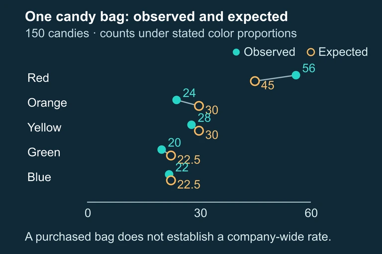 Observed color counts from one purchased bag can be compared with the stated model, but this design does not establish company-wide inference.
Five-category, 150-candy illustration. This does not replace the separate six-category, 200-candy worked example.
SECTION 7
Common Errors & Best Practices
Students frequently lose points on AP free-response questions not because they cannot calculate χ², but because they make procedural or interpretive mistakes. The table below contrasts common errors with the corresponding best practices. Internalizing these distinctions can make the difference between partial and full credit.
| Common Error | Best Practice | Why It Matters |
|---|---|---|
| Using proportions instead of counts in the formula | Always use raw counts (O and E) in the χ² formula, not percentages or proportions | The formula requires counts; using proportions yields an incorrect (too small) χ² value |
| Using observed counts in the denominator: (O − E)²/O | The denominator is always the expected count E, not the observed count O | Standardization by E is what connects the statistic to the χ² distribution |
| Saying 'accept H₀' instead of 'fail to reject H₀' | Use 'fail to reject H₀'—a non-significant result does not prove H₀ is true | Accepting H₀ implies certainty that H₀ is true, which is logically unjustified |
| Failing to state the conclusion in context | Always reference the specific categorical variable and population in your conclusion | The AP rubric requires contextual language—generic conclusions lose points |
| Computing a two-tailed p-value | The chi-square GOF test is always right-tailed; large χ² values provide evidence against H₀ | The chi-square distribution is not symmetric, so 'two-tailed' has no meaning here |
Common errors and best practices for chi-square goodness-of-fit tests
KEY TAKEAWAY
SECTION 8
Connection to Other Chi-Square Tests
The chi-square goodness-of-fit test is one member of a family of chi-square procedures. All three share the same test statistic formula—Σ(O − E)²/E—but they differ in the research question, the data structure, and the degrees of freedom. Understanding these distinctions helps you select the correct test on the AP Exam and in practice.
| Feature | Goodness of Fit | Test of Independence | Test of Homogeneity |
|---|---|---|---|
| Number of variables | One categorical variable | Two categorical variables, one sample | One categorical variable across multiple populations |
| H₀ | Distribution matches a specified model | The two variables are independent | The distribution is the same across populations |
| Data structure | One-way frequency table | Two-way contingency table | Two-way contingency table |
| Degrees of freedom | k − 1 | (r − 1)(c − 1) | (r − 1)(c − 1) |
| Expected counts from | n × p₀ᵢ (hypothesized proportions) | (row total × column total) / n | (row total × column total) / n |
Comparison of the three chi-square tests in AP Statistics
As you progress through the chi-square unit, you will see that mastering the goodness-of-fit procedure gives you a strong foundation for the other two tests. The computational machinery is identical; only the source of expected counts and the interpretation of the hypotheses change. In more advanced coursework, you may encounter likelihood-ratio tests (G-tests), which use a different formula to measure discrepancy but follow the same logical framework. The Pearson chi-square statistic remains the standard approach in introductory statistics courses and on the AP Exam because it is intuitive, computationally accessible, and performs well under the conditions typically encountered in practice.
SECTION 9
Practice Problems
Question 1: CONCEPTUAL
- A. The observed counts are exactly equal to the expected counts in all 5 categories.
- B. There is convincing evidence that the distribution differs from the hypothesized model.
- C. The observed counts differ only slightly from the expected counts, and the differences are consistent with random sampling variability.
- D. The hypothesized distribution has been proven to be correct.
- E. The test is invalid because χ² must be at least 5 to draw any conclusion.
Show answer (C)
Question 2: BASIC CALCULATION
- A. χ² = 0.12
- B. χ² = 0.48
- C. χ² = 0.84
- D. χ² = 1.20
- E. χ² = 3.00
Show answer (B)
Question 3: INTERMEDIATE
- A. Because χ² = 14.00 > 13.28, the p-value < 0.01, so we reject H₀. There is convincing evidence that complaints are not equally distributed across weekdays.
- B. Because χ² = 14.00 > 13.28, the p-value > 0.01, so we fail to reject H₀.
- C. Because χ² = 14.00 < 16, we cannot reject H₀ at any significance level.
- D. We accept H₀ and conclude the distribution is uniform because the difference is small.
- E. The test is inconclusive because the expected count for each day is 16, which is close to several observed counts.
Show answer (A)
Question 4: APPLIED
4 ptsShow answer
Question 5: CRITICAL THINKING
4 ptsShow answer
SUMMARY
Summary
Summary
The chi-square goodness-of-fit test evaluates whether the distribution of a single categorical variable matches a hypothesized model. You compute expected counts as Eᵢ = n × p₀ᵢ, then calculate the test statistic χ² = Σ(Oᵢ − Eᵢ)²/Eᵢ, which measures the total standardized discrepancy between observed and expected counts across all k categories. The test uses df = k − 1 degrees of freedom, and the p-value is always computed from the right tail of the chi-square distribution.
A complete AP-level response includes: stating hypotheses, verifying that all expected counts are at least 5 and the sample is random, showing the formula and computed value of χ², reporting the p-value with df, comparing it to α, and stating a conclusion in context using appropriate language of evidence. Remember: you reject H₀ when the p-value < α, and you fail to reject (never 'accept') H₀ otherwise. Examining which categories contribute the most to χ² reveals where the hypothesized model fits poorly.