Setting Up a Chi-Square Goodness of Fit Test - AP Statistics

SECTION 1

Historical Context & Motivation

Statistical inference about categorical data poses a fundamentally different challenge than inference about means or proportions. When a researcher observes counts spread across multiple categories—such as the number of customers choosing each of six flavors—the question is not whether a single parameter equals some value, but whether an entire distribution of proportions matches a theoretical model. The tool built precisely for this purpose is the chi-square goodness of fit test, and understanding how to set it up correctly is the critical first step in applying it.

1900 • Pearson's Chi-Square Statistic

Karl Pearson published the chi-square statistic as a way to measure the discrepancy between observed frequencies and frequencies expected under a theoretical model. His paper in the Philosophical Magazine laid the foundation for modern categorical inference.

1922 • Fisher's Refinement

Ronald Fisher clarified the correct degrees of freedom for the chi-square distribution and distinguished between cases where parameters are known versus estimated from data, formalizing the inferential framework.

1952 • Cochran's Sample-Size Guidelines

William Cochran established the widely cited rule that expected counts should be at least 5 in every cell, giving practitioners a practical condition for when the chi-square approximation is reliable.

2000s • Modern AP Statistics Curriculum

The College Board's AP Statistics course formalized the four-step inference process—state, plan, do, conclude—making the setup of a chi-square goodness of fit test a cornerstone topic in the exam framework.

The central question the goodness of fit test addresses is deceptively simple: Do the observed counts in a set of categories differ significantly from what a hypothesized distribution predicts? Before any calculation takes place, the test must be set up with precise hypotheses, verified conditions, and a clear identification of the appropriate distribution. Getting the setup wrong can invalidate everything that follows, which is why the AP exam devotes considerable attention to this preliminary phase.

SECTION 2

Core Principles & Definitions

Setting up a chi-square goodness of fit test requires mastery of several interconnected ideas. The test applies to a single categorical variable whose outcomes fall into k mutually exclusive categories. The null hypothesis specifies an exact set of proportions for those categories, and the alternative hypothesis asserts that at least one proportion deviates from its hypothesized value. The following grid outlines the foundational concepts you need before writing a single symbol.

Observed Counts (O)

The actual frequencies recorded in each category from your sample data. These are the raw counts you collect, not proportions or percentages.

Expected Counts (E)

The frequencies you would expect in each category if the null hypothesis were true. Computed as E = n × p_i, where n is the total sample size and p_i is the hypothesized proportion for category i.

Null Hypothesis (H₀)

A precise claim that the population distribution of the categorical variable matches a specified set of proportions. All k proportions must be stated and must sum to 1.

Alternative Hypothesis (Hₐ)

The claim that at least one of the population proportions differs from the value stated in H₀. Note: this is always nondirectional—you never specify which category deviates.

Conditions for Inference

Three conditions must be verified: (1) Random — data come from a random process; (2) Independence — the 10% condition or sampling with replacement; (3) Large Counts — every expected count is at least 5.

✦

KEY TAKEAWAY

Think of the null hypothesis as a blueprint for a mosaic. The blueprint says exactly how much area each colored tile should cover. The goodness of fit test checks whether the actual mosaic you observe matches that blueprint closely enough—or whether the discrepancies are too large to attribute to random variation in tile placement. The setup phase is where you lay out the blueprint and verify you have enough tiles (sample size) to make a meaningful comparison.

SECTION 3

Visual Explanation: The Setup Flowchart

The flowchart above summarizes the three setup phases of a chi-square goodness of fit test: stating hypotheses with all k proportions, verifying the Random, Independence, and Large Counts conditions, and identifying the test name along with its degrees of freedom (df = k − 1).

The flowchart captures the entire setup process that should appear in the State and Plan stages of the AP Statistics four-step inference process. In the State step, you write both hypotheses and define the parameter in context—the distribution of a categorical variable in the population. In the Plan step, you name the procedure, verify the three conditions, and note the degrees of freedom. Only after these steps are complete do you proceed to calculate the test statistic and draw a conclusion.

SECTION 4

Mathematical Framework

Although the focus of this lesson is the setup, understanding the formula you are setting up to use clarifies why each piece of the setup matters. The chi-square test statistic quantifies the overall discrepancy between observed and expected counts, and its sampling distribution under H₀ is approximately chi-square with k − 1 degrees of freedom—provided the conditions are met.

CHI-SQUARE TEST STATISTIC

χ² = Σ (Oᵢ − Eᵢ)² / Eᵢ

Where Oᵢ = observed count for category i, Eᵢ = expected count for category i = n × p_i, and the sum is taken over all k categories.

EXPECTED COUNT FORMULA

Eᵢ = n × pᵢ

Where n = total sample size and pᵢ = the proportion specified for category i in H₀. Computing expected counts is part of the setup because you must verify the Large Counts condition before proceeding.

DEGREES OF FREEDOM

df = k − 1

Where k = the number of categories. One degree of freedom is lost because the proportions must sum to 1, so the last proportion is determined once the others are known.

⚠

Why Expected Counts ≥ 5?

The chi-square test statistic follows an approximate χ² distribution only when sample sizes are large enough. When any expected count falls below 5, the chi-square approximation deteriorates because the sampling distribution of (O − E)²/E becomes too skewed. Checking this condition during setup prevents you from drawing invalid conclusions later.

SECTION 5

Writing Hypotheses & Checking Conditions in Detail

The most common errors students make on the AP exam involve the hypotheses and conditions. This section breaks down every component so that your setup earns full credit. When writing hypotheses, you must define the parameter in the context of the problem. A generic statement like "the data fit the model" is not sufficient; you need to state what the categorical variable represents and specify every proportion.

This diagram annotates a model setup with four categories, showing exactly what to write for the State and Plan phases. Notice that the null hypothesis lists every proportion, the conditions are verified with context-specific evidence, and the test is named with its degrees of freedom.

Common Pitfalls in the Setup

Omitting proportions from H₀ — Writing "H₀: the distribution is uniform" without specifying each pᵢ = 1/k will cost you credit. Always list the numerical values.
Using proportions instead of counts for the Large Counts check — The condition is about expected counts (E ≥ 5), not expected proportions. Compute E = n × p for each category.
Stating Hₐ as directional — The chi-square test is inherently one-sided (right-tail only), but Hₐ should state "at least one proportion differs," not specify which one is larger or smaller.
Confusing observed and expected counts — The Large Counts condition requires expected counts ≥ 5, not observed counts. Even if an observed count is 2, the test may still be valid if the expected count is ≥ 5.

SECTION 6

Worked Example: Setting Up a Goodness of Fit Test

A candy company claims that its mixed bag contains 30% red, 20% orange, 20% yellow, 15% green, and 15% blue candies. A statistics student purchases a bag, selects a simple random sample of 150 candies, and records the following observed counts: 56 red, 24 orange, 28 yellow, 20 green, and 22 blue. The student wants to test whether the company's claimed distribution is accurate at the α = 0.05 significance level.

Setting Up the Chi-Square Goodness of Fit Test

1
Step 1 — Define the Parameter

Let the parameter be the true distribution of candy colors in the company's mixed bags. We are examining a single categorical variable (color) with five categories.
2
Step 2 — State the Hypotheses

H₀: The distribution of candy colors is p_red = 0.30, p_orange = 0.20, p_yellow = 0.20, p_green = 0.15, p_blue = 0.15. Hₐ: At least one of the proportions of candy colors differs from its stated value.

Hypotheses stated with all five proportions summing to 1.00.
3
Step 3 — Name the Test and Significance Level

We will perform a chi-square goodness of fit test at α = 0.05. The degrees of freedom are df = k − 1 = 5 − 1 = 4.

df = 4, α = 0.05
4
Step 4 — Check the Random Condition

The stated simple random sample is drawn within one purchased bag. This supports randomness within that bag, not an SRS across company production. Company-wide inference needs a sampling design that represents the company population.

Within-bag randomness is stated; company-wide representativeness is not established.
5
Step 5 — Check the Independence Condition

For sampling without replacement from the bag, check 150 ≤ 10% of the number of candies in that bag, which requires at least 1,500 candies. Company production size is not the relevant frame for this sample. The bag size is not given, and an appropriate independence or multinomial model must be justified before using the usual chi-square reference distribution.

Independence requires additional information about the bag and sampling process.
6
Step 6 — Check the Large Counts Condition

Compute expected counts under H₀: E_red = 150 × 0.30 = 45, E_orange = 150 × 0.20 = 30, E_yellow = 150 × 0.20 = 30, E_green = 150 × 0.15 = 22.5, E_blue = 150 × 0.15 = 22.5. All expected counts are at least 5, so the Large Counts condition is satisfied.

✔ All expected counts ≥ 5 (smallest is 22.5).
7
Step 7 — Summary of Setup

The expected-count condition holds, with expected counts 45, 30, 30, 22.5 and 22.5. The hypotheses and df = 4 are specified, but the random-sampling and independence limitations above remain. A chi-square calculation could be performed conditionally on justified assumptions; these data alone do not establish a valid company-wide test.

Setup identifies the model and its unresolved sampling assumptions.

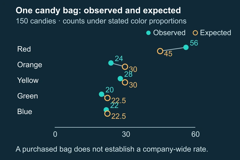Five observed versus expected candy counts for a 150-candy example. Expected counts include 45,30,30,22.5,22.5. Sampling from one bag does not establish company-wide inference. Observed color counts from one purchased bag can be compared with the stated model, but this design does not establish company-wide inference.

The five-category, 150-candy setup; company-wide inference is not established by one bag.

SECTION 7

Strengths & Limitations of the Goodness of Fit Test

The chi-square goodness of fit test is one of the most versatile tools in the categorical inference toolkit, but it has important limitations that shape how you set it up and interpret its results. The table below contrasts its key strengths against scenarios where caution is required.

Strengths	Limitations
Works with any number of categories (k ≥ 2), making it flexible for nominal and ordinal data alike.	Requires all expected counts to be at least 5; when categories have small expected counts, you may need to combine categories or use an exact test.
The null hypothesis can specify any distribution—uniform, historical, theoretical—not just equal proportions.	The test is omnibus: a significant result tells you the distribution differs from H₀ but does not identify which specific categories deviate.
Computation is straightforward and supported by all major calculators and software packages.	The test uses counts, not proportions. Entering proportions or percentages into the formula produces incorrect results.
Minimal distributional assumptions—no requirement of normality for the underlying variable.	Independence is assumed; repeated measures or clustered data violate this condition and require alternative methods.

Strengths and limitations of the chi-square goodness of fit test

✦

KEY TAKEAWAY

The goodness of fit test is like a quality-control inspector who can tell you that something in a shipment doesn't match the specification—but the inspector checks the entire shipment as a unit, not each item individually. When the alarm goes off (small p-value), you know the overall distribution is off, but you need follow-up analysis (examining individual contributions to χ²) to pinpoint which categories are responsible.

SECTION 8

Connections to Other Chi-Square Tests

The goodness of fit test is one of three chi-square procedures in the AP Statistics curriculum. Understanding how it relates to the chi-square test for independence and the chi-square test for homogeneity clarifies when to use each and how the setup differs across the three tests.

Feature	Goodness of Fit	Test for Independence / Homogeneity
Number of variables	One categorical variable	Two categorical variables (arranged in a two-way table)
Data layout	One-way frequency table (single row or column of counts)	Two-way contingency table (r rows × c columns)
H₀ statement	The population distribution matches specified proportions	The two variables are independent / the distributions are the same across populations
Expected counts	E = n × p (from hypothesized proportions)	E = (row total × column total) / grand total
Degrees of freedom	k − 1	(r − 1)(c − 1)

Comparison of chi-square procedures in AP Statistics

Notice that all three tests share the same test statistic formula, χ² = Σ (O − E)²/E, and the same Large Counts condition (all expected counts ≥ 5). The key difference lies in how expected counts are computed and how degrees of freedom are determined. In the goodness of fit test, the expected counts come directly from the hypothesized proportions multiplied by n, whereas in the two-way tests, they are derived from marginal totals. As you move through the AP curriculum, mastering the goodness of fit setup provides the template for the more complex two-variable setups.

SECTION 9

Practice Problems

Question 1: CONCEPTUAL

A researcher wants to test whether the distribution of blood types (A, B, AB, O) in a city matches the national distribution. Which of the following is the correct alternative hypothesis for a chi-square goodness of fit test?

A. Hₐ: $p_A$ ≠ 0.36, $p_B$ ≠ 0.28, p_AB ≠ 0.08, $p_O$ ≠ 0.28
B. Hₐ: At least one of the proportions of blood types in the city differs from the national distribution.
C. Hₐ: The distribution of blood types in the city is uniform.
D. Hₐ: The mean blood type proportion is not equal to 0.25.
E. Hₐ: $p_A$ > 0.36 or $p_B$ > 0.28 or p_AB > 0.08 or $p_O$ > 0.28

Show answer (B)

B is correct. The alternative hypothesis for a chi-square goodness of fit test is always stated as "at least one proportion differs from its hypothesized value." Choice A is wrong because it claims every proportion differs, which is too specific; the test only requires at least one to differ. Choice C describes a different null hypothesis (uniform distribution) and is not an alternative. Choice D incorrectly references means; the chi-square test deals with categorical proportions, not means. Choice E introduces directional inequalities, but the goodness of fit test is not directional in that sense—it detects any deviation from the specified distribution.

Question 2: BASIC CALCULATION

A store claims that 40% of its sales come from online orders, 35% from in-store purchases, and 25% from phone orders. A random sample of 200 sales is taken. What is the expected count for phone orders under H₀, and how many degrees of freedom does this test have?

A. Expected count = 50, df = 2
B. Expected count = 50, df = 3
C. Expected count = 25, df = 2
D. Expected count = 0.25, df = 2
E. Expected count = 50, df = 199

Show answer (A)

A is correct. The expected count for phone orders is E = n × p = 200 × 0.25 = 50. The degrees of freedom are df = k − 1 = 3 − 1 = 2. Choice B incorrectly uses df = k = 3 instead of k − 1. Choice C confuses the percentage (25) with the expected count—you must multiply the proportion by n. Choice D uses the proportion (0.25) itself rather than computing n × p. Choice E uses n − 1 = 199, which is the degrees of freedom for a t-test, not a chi-square goodness of fit test.

Question 3: INTERMEDIATE

A biologist believes that a particular gene produces phenotypes in a 9:3:3:1 ratio. She observes 120 organisms. Which of the following correctly states the expected counts and the Large Counts condition check?

A. E₁ = 67.5, E₂ = 22.5, E₃ = 22.5, E₄ = 7.5; all expected counts ≥ 5, condition met.
B. E₁ = 67.5, E₂ = 22.5, E₃ = 22.5, E₄ = 7.5; the condition fails because 7.5 is not a whole number.
C. E₁ = 30, E₂ = 30, E₃ = 30, E₄ = 30; all expected counts ≥ 5, condition met.
D. E₁ = 9, E₂ = 3, E₃ = 3, E₄ = 1; the condition fails because 1 < 5.
E. E₁ = 67.5, E₂ = 22.5, E₃ = 22.5, E₄ = 7.5; the condition fails because we need observed counts ≥ 5.

Show answer (A)

A is correct. The 9:3:3:1 ratio means proportions of 9/16, 3/16, 3/16, and 1/16. Expected counts: 120 × 9/16 = 67.5, 120 × 3/16 = 22.5, 120 × 3/16 = 22.5, and 120 × 1/16 = 7.5. All are ≥ 5, so the Large Counts condition is satisfied. Choice B is wrong because expected counts do not need to be whole numbers—they represent theoretical averages. Choice C incorrectly assumes a uniform distribution rather than the 9:3:3:1 ratio. Choice D uses the ratio values (9, 3, 3, 1) directly as expected counts instead of computing n × (ratio/total). Choice E confuses observed counts with expected counts; the Large Counts condition checks expected counts, not observed.

Question 4: APPLIED

5 pts

A transportation planner collected a random sample of 300 commuters from a metropolitan area and recorded their primary mode of transportation. The planner wants to test whether the distribution of commuting modes matches a model derived from a national survey. The national model claims: drive alone = 0.76, carpool = 0.09, public transit = 0.05, walk = 0.03, work from home = 0.05, other = 0.02. Set up the complete hypothesis test: state hypotheses, verify all conditions, and identify the test with its degrees of freedom. Show all expected counts.

Show answer

Rubric (5 points): Point 1 — Hypotheses (1 pt): H₀: The distribution of commuting modes in the metro area is p(drive alone) = 0.76, p(carpool) = 0.09, p(public transit) = 0.05, p(walk) = 0.03, p(work from home) = 0.05, p(other) = 0.02. Hₐ: At least one of the proportions of commuting modes differs from its stated value. Proportions must sum to 1.00 and be stated in context. Point 2 — Random condition (1 pt): The problem states the planner collected a random sample of 300 commuters, satisfying the Random condition. Point 3 — Independence condition (1 pt): 300 commuters is less than 10% of all commuters in a metropolitan area (reasonable to assume N > 3,000). The 10% condition is satisfied. Point 4 — Large Counts condition with all expected counts shown (1 pt): E(drive alone) = 300 × 0.76 = 228; E(carpool) = 300 × 0.09 = 27; E(public transit) = 300 × 0.05 = 15; E(walk) = 300 × 0.03 = 9; E(work from home) = 300 × 0.05 = 15; E(other) = 300 × 0.02 = 6. All expected counts are ≥ 5, so the Large Counts condition is satisfied. Point 5 — Test identification (1 pt): We will use a chi-square goodness of fit test with df = 6 − 1 = 5 at the chosen significance level. Note: if the "other" expected count of 6 is the smallest, the condition is still met (6 ≥ 5). A complete response identifies the test name and computes the correct degrees of freedom.

Question 5: CRITICAL THINKING

4 pts

A sociologist surveys a random sample of 80 households and classifies each into one of five income brackets. The hypothesized distribution is: under $30K = 0.20, $30K–$60K = 0.30, $60K–$90K = 0.25, $90K–$120K = 0.15, over $120K = 0.10. (a) Verify whether the Large Counts condition is satisfied. (b) If the condition is not satisfied for some category, explain two possible strategies the sociologist could use so that the chi-square goodness of fit test can still be performed. (c) Discuss how combining categories might affect the interpretation of the test results.

Show answer

Rubric (4 points): Point 1 — Large Counts verification (1 pt): Expected counts: E₁ = 80 × 0.20 = 16; E₂ = 80 × 0.30 = 24; E₃ = 80 × 0.25 = 20; E₄ = 80 × 0.15 = 12; E₅ = 80 × 0.10 = 8. All expected counts are ≥ 5, so the Large Counts condition is satisfied with this sample size. However, if the sample were smaller (e.g., n = 40), E₅ = 4 and the condition would fail. Point 2 — Strategy 1: Increase sample size (1 pt): If any expected count were below 5, the sociologist could collect a larger sample. Since E = n × p, increasing n raises every expected count proportionally. The minimum sample size needed can be found by setting n × p(min) ≥ 5, so n ≥ 5/p(min). For p = 0.10, this gives n ≥ 50. Point 3 — Strategy 2: Combine categories (1 pt): The sociologist could merge adjacent categories with small expected counts into a single category. For example, combining "$90K–$120K" and "over $120K" into "over $90K" with a combined proportion of 0.25 would yield E = n × 0.25, which is larger and more likely to satisfy the condition. Point 4 — Impact on interpretation (1 pt): Combining categories reduces the number of categories (k), which lowers the degrees of freedom and changes the null hypothesis being tested. The new test can only detect whether the distribution matches the combined model, not whether each original category's proportion is correct individually. Specifically, if the original two categories each deviated from their hypothesized proportions but in opposite directions, the deviations could cancel when combined, reducing the power of the test to detect that particular pattern of deviation. The researcher loses granularity and may miss important distributional differences within the merged group.

SUMMARY

Lesson Summary

Summary

Setting up a chi-square goodness of fit test begins with clearly stating the null hypothesis, which specifies a complete set of population proportions for each category of a single categorical variable, and the alternative hypothesis, which asserts that at least one proportion differs. Every proportion must be listed explicitly, and they must sum to 1. The parameter should be defined in the context of the problem.

Before computing anything, you must verify three conditions: the Random condition (data come from a random sample or random process), the Independence condition (sample size is less than 10% of the population), and the Large Counts condition (all expected counts E = n × p ≥ 5). Finally, identify the procedure as a chi-square goodness of fit test with df = k − 1 degrees of freedom. Mastering this setup ensures a solid foundation for the Do and Conclude steps that follow.