Analyzing Departures from Linearity - AP Statistics

SECTION 1

Historical Context & Motivation

The idea of fitting a straight line through data goes back to the early nineteenth century, when least-squares regression was independently developed by Adrien-Marie Legendre and Carl Friedrich Gauss to predict the orbits of celestial bodies. For over a century, practitioners applied linear models almost reflexively, rarely pausing to verify whether the assumed straight-line form was actually appropriate. It was only as data sets grew larger and computational tools became available that statisticians recognized the need for systematic diagnostics that could reveal when a linear model was misleading rather than informative.

1805 • Legendre's Least Squares

Adrien-Marie Legendre publishes the method of least squares, providing the first formal algorithm for fitting a linear model to bivariate data.

1885 • Galton's Regression to the Mean

Francis Galton introduces 'regression toward mediocrity' in his study of heights, establishing the concept of the regression line and spurring interest in how well linear models capture real relationships.

1973 • Anscombe's Quartet

Frank Anscombe constructs four data sets sharing identical regression statistics (slope, intercept, r²) yet displaying wildly different scatter patterns—dramatically demonstrating that numerical summaries alone cannot confirm linearity.

1977 • Tukey's EDA Movement

John Tukey's Exploratory Data Analysis formalizes the principle of 'looking at the data first,' championing residual plots and other graphical diagnostics as standard practice.

The central question this lesson addresses is deceptively simple: after you fit a line, how do you know whether the line is actually a good description of the relationship? As Anscombe's Quartet powerfully illustrates, summary statistics like r and r² can mask severe departures from linearity, making graphical residual analysis an indispensable skill for any practicing statistician.

SECTION 2

Core Principles & Definitions

Before diagnosing departures from linearity, you must be fluent in several foundational concepts that underpin residual analysis. A residual is defined as the difference between an observed response value and the value predicted by the regression line: e = y − ŷ. Residuals are the diagnostic currency of regression—they encode every piece of information the model failed to capture. When the linear model is appropriate, residuals should appear structureless; any visible pattern suggests the model is inadequate.

Residual Plot

A scatterplot of residuals (e) on the vertical axis against the explanatory variable (x) or fitted values (ŷ) on the horizontal axis. A well-fitting linear model yields a residual plot with no discernible pattern—only random scatter centered on zero.

Curvature (Nonlinearity)

When the residual plot shows a systematic curved pattern—typically a U-shape or inverted U—the true relationship between x and y is nonlinear, and the straight-line model systematically over- and under-predicts in different regions.

Non-Constant Spread (Heteroscedasticity)

If the vertical spread of residuals fans out (or funnels in) as x increases, the variability of the response is not constant across the range of x, violating a key regression assumption and distorting inference.

Influential Points & Outliers

Points with unusually large residuals (outliers) or extreme x-values (high leverage) can disproportionately shift the regression line. Identifying them is critical before drawing conclusions from any fitted model.

Coefficient of Determination (r²)

r² measures the proportion of variability in y explained by the linear model. A high r² is necessary but not sufficient for linearity—a curved relationship can still produce a high r² while being poorly modeled by a line.

✦

KEY TAKEAWAY

Think of fitting a regression line like using a ruler to trace the path of a winding river on a map. The ruler captures the general direction, but the bends and meanders are lost. Residuals measure precisely how far the river departs from the ruler at every point. If the residuals show a pattern of systematic departures rather than random wobble, the ruler is the wrong tool—you need a flexible curve.

SECTION 3

Residual Plots — The Visual Diagnostic

The single most powerful tool for detecting departures from linearity is the residual plot. The diagram below contrasts three scenarios: a residual plot consistent with a good linear fit, one showing systematic curvature, and one exhibiting non-constant spread. Study the shapes carefully—recognizing these patterns at a glance is essential on the AP exam.

Left: Residuals scatter randomly about the zero line with roughly constant spread—evidence that a linear model is appropriate. Center: A clear U-shaped (or inverted-U) pattern indicates curvature in the original data; the linear model systematically overestimates in the middle and underestimates at the extremes. Right: A fan-shaped spread signals heteroscedasticity, where variability in y increases with x.

When reading a residual plot, focus on two questions. First, is there a systematic shape (curve, wave, or cluster) rather than formless scatter? If so, the linear model is missing a structural feature of the data. Second, does the vertical spread remain roughly the same from left to right? Increasing or decreasing spread (the 'fan' or 'funnel' pattern) indicates that precision of prediction varies across the range of x, which undermines standard inference procedures that assume constant variance.

SECTION 4

Mathematical Framework

The least-squares regression line minimizes the sum of squared residuals. Understanding the formal definitions clarifies exactly what residuals measure and why their behavior reveals model inadequacy.

LEAST-SQUARES REGRESSION LINE

ŷ = b₀ + b₁x

where ŷ is the predicted response, b₀ is the y-intercept, and b₁ is the slope. The slope b₁ = r × (s_y / s_x), and the line always passes through (x̄, ȳ).

RESIDUAL DEFINITION

eᵢ = yᵢ − ŷᵢ

A positive residual means the observed value lies above the regression line (model underestimates), while a negative residual means the observed value lies below (model overestimates). The sum of all residuals for an LSRL equals zero: Σeᵢ = 0.

COEFFICIENT OF DETERMINATION

r² = 1 − (SSE / SST)

SSE = Σ(yᵢ − ŷᵢ)² is the sum of squared residuals. SST = Σ(yᵢ − ȳ)² is the total sum of squares. r² gives the proportion of variation in y explained by the linear model. A high r² does not guarantee linearity—it only measures how much spread is reduced by the model.

STANDARD DEVIATION OF RESIDUALS

s = √[Σeᵢ² / (n − 2)]

Also called the residual standard error, s estimates the typical size of a prediction error. A smaller s indicates predictions are, on average, closer to observed values. We divide by n − 2 because fitting a line consumes two degrees of freedom (one for the slope, one for the intercept).

💡

AP Exam Tip

On the AP Statistics exam, you will frequently be asked to interpret a residual plot and state whether a linear model is appropriate. Always reference the specific pattern you observe—'there is a curved pattern in the residual plot, indicating the relationship is not linear'—rather than simply saying 'the residual plot looks bad.'

SECTION 5

Detailed Diagnostic Breakdown

Beyond recognizing gross patterns, effective residual analysis requires distinguishing among several specific types of departures. The diagram below illustrates additional diagnostic scenarios, including the effect of outliers and influential observations. The accompanying classification table provides a quick-reference guide for interpreting what you see.

The left panel shows a scatterplot where points follow a curve (green) but a straight line (red dashed LSRL) has been fitted. The data might appear 'roughly linear' at first glance, especially with a moderate r². The right panel plots the residuals from that LSRL—the U-shaped pattern unmistakably reveals the curvature that was partially hidden in the original plot.

Residual Plot Pattern	Diagnosis	Action / Remedy
Random scatter, roughly constant spread around e = 0	Linear model is appropriate	Proceed with inference; report slope, r², and s
Curved (U-shape or inverted-U)	Nonlinear relationship; line misses the true pattern	Try a transformation (e.g., log, square root, power) or fit a polynomial/exponential model
Fan or funnel shape (spread changes with x)	Heteroscedasticity (non-constant variance)	Consider a log transformation on y or use weighted regression
One or two points far from the rest	Outlier (large residual) or influential point (high leverage)	Investigate cause; refit without the point and compare results
Clusters or grouping in residuals	Possible lurking variable creating subgroups	Stratify by the grouping variable and fit separate models, or add the variable to a multiple regression model

Residual plot pattern interpretation guide

SECTION 6

Worked Example

A biologist records age (years) and trunk diameter (centimeters) for seven oak trees. The least-squares line is ŷ = 8.9285714286 + 1.2642857143x, with R² ≈ 0.99463458. The table gives predictions and residuals from that fit. Determine what these data do and do not establish about a linear model.

Age (x)	Diameter (y)	Predicted (ŷ)	Residual (e)
5	14.0	15.250	−1.250
10	22.5	21.571	+0.929
15	28.0	27.893	+0.107
20	35.0	34.214	+0.786
25	40.0	40.536	−0.536
30	48.0	46.857	+1.143
35	52.0	53.179	−1.179

Seven oak trees; predictions and residuals from ŷ = 8.9285714286 + 1.2642857143x, rounded to three decimals.

Analyzing the Oak Tree Residuals

1
Step 1 — Examine r²

R² ≈ 0.99463458 means this fitted line accounts for about 99.46% of the observed diameter variation. A high R² alone does not confirm linearity; examine the residuals and the limited sample size.
2
Step 2 — Construct the Residual Plot (mentally or on calculator)

At ages 5,10,15,20,25,30,35, the residuals are approximately −1.250,+0.929,+0.107,+0.786,−0.536,+1.143,−1.179 cm. They sum to zero apart from rounding. Both positive and negative residuals occur across the age range; they do not follow a transition from positive values to increasingly negative ones.
3
Step 3 — Identify the Pattern

These seven residuals do not establish the previously suggested monotonic curvature. Inspecting their plotted shape is still useful, but the small sample limits conclusions about model form. A high R² and a short residual series cannot certify that the population relationship is exactly linear.

No established monotonic curvature; seven points limit the diagnosis.
4
Step 4 — State the Conclusion

The fitted line closely summarizes these seven observed pairs. The residuals do not justify rejecting it on the basis of the claimed monotonic pattern or automatically applying a transformation. Continue to check model assumptions and gather more data when prediction matters; high R² alone is not sufficient validation.

Retain a provisional linear summary; do not force an unsupported transformation.

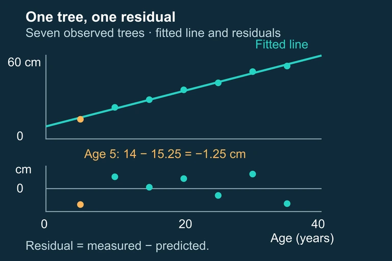
Seven oak-tree age/diameter pairs with their fitted line and aligned residual plot. The residual at age 5 is −1.25 cm. Seven oak measurements determine the fitted line and residuals. Each residual is the observed diameter minus its predicted diameter; the small sample does not establish a unique growth law. The field scene illustrates circumference measurement; the supplied diameter records are the regression data, rather than values inferred from the picture.

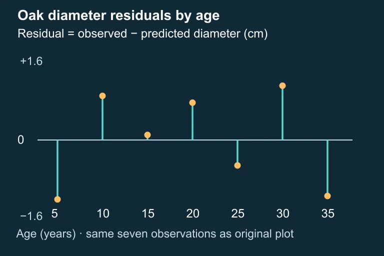
Residuals for seven oak trees at ages 5 through 35, plotted around a common zero line within ±1.6 cm.

SECTION 7

Strengths & Limitations of Residual Analysis

Strengths	Limitations
Residual plots can reveal curvature, non-constant spread, and outliers that summary statistics like r² completely miss.	With small sample sizes, random variation can mimic patterns, making it difficult to distinguish real departures from noise.
The technique requires no additional data collection—residuals are automatically produced by any regression software or graphing calculator.	Residual analysis is inherently subjective; two analysts may disagree about whether a pattern is 'systematic enough' to matter.
Residual plots are intuitive and communicate results visually, making them effective for both analysis and presentation.	A clean residual plot does not prove the model is correct—it only fails to reveal a problem. There may be lurking variables or issues not captured by a single predictor.
Identifying influential points via large residuals can flag data entry errors or unusual observations that deserve further investigation.	High-leverage points may not have large residuals precisely because they pull the line toward themselves, masking their own influence.

Strengths and limitations of residual analysis for detecting departures from linearity

✦

KEY TAKEAWAY

Residual analysis is like a quality-control inspection on an assembly line. Passing inspection (no pattern in residuals) does not guarantee a flawless product, but failing inspection (clear pattern) provides an unambiguous signal that something is wrong with the manufacturing process. In statistics, 'something is wrong' means the linear model is not capturing the true relationship, and you should investigate further before reporting results.

SECTION 8

Connecting to Transformations & Advanced Models

When residual analysis reveals a departure from linearity, the natural next step is to transform the data so that the relationship between the transformed variables is approximately linear. This strategy is central to the AP Statistics curriculum and connects residual diagnostics to a broader toolkit of modeling techniques. The two most common transformations—logarithmic and power—address the two most common types of curved relationships: exponential growth/decay and power functions.

Feature	Linear Model (no transform)	Log Transformation	Power Transformation
Form of equation	ŷ = b₀ + b₁x	log(ŷ) = a + bx → ŷ = 10ᵃ × 10ᵇˣ	log(ŷ) = a + b·log(x) → ŷ = 10ᵃ × xᵇ
Typical pattern in original residual plot	Random scatter (model is fine)	Exponential curve; residuals accelerate	Concave-down curve; residuals level off
What to plot for linearity check	y vs. x	log(y) vs. x	log(y) vs. log(x)
When to try it	Residual plot shows no pattern	Data show multiplicative (percentage) growth	Data follow a physical/biological scaling law

Comparing the linear model with common transformations used to address departures from linearity

In more advanced statistics courses, you will encounter polynomial regression, spline smoothing, and generalized additive models that handle nonlinearity without requiring you to choose a specific transformation. However, at the AP level, the critical skill is recognizing when the linear model fails via the residual plot and knowing that a logarithmic or power transformation may restore linearity. In the free-response section, clearly stating the evidence (the pattern in the residual plot) and the remedy (a specific transformation) demonstrates the kind of structured reasoning that earns full credit.

SECTION 9

Practice Problems

Question 1: CONCEPTUAL

A student fits a least-squares regression line to a bivariate data set and obtains r² = 0.95. The student claims that because r² is very high, a linear model is definitely appropriate. Which of the following best explains why this reasoning is flawed?

A. A high r² only indicates the slope is steep; it says nothing about the form of the relationship.
B. A high r² means the data are approximately normal, not necessarily linear.
C. A nonlinear relationship (such as a quadratic) can still produce a high r², so a residual plot must be checked for patterns before concluding linearity is appropriate.
D. r² cannot exceed 0.90 for data that are truly linear, so a value of 0.95 actually suggests nonlinearity.
E. The student should have used the correlation coefficient r instead of r², since r is more sensitive to departures from linearity.

Show answer (C)

The correct answer is C. r² measures the proportion of variability in y explained by the linear model, but a strong curved relationship (e.g., quadratic or exponential) can also produce a high r² because the curve is close to a line over much of its range. Anscombe's Quartet famously demonstrates that data sets with identical r² values can have vastly different shapes. A is wrong because r² measures strength of the linear relationship, not the steepness of slope. B is wrong because r² has nothing to do with normality of the data. D is wrong because there is no upper bound on r² for linear data—perfectly linear data yield r² = 1. E is wrong because r and r² contain the same information about the linear fit; neither one alone can detect nonlinearity without a residual plot.

Question 2: BASIC CALCULATION

A regression analysis produces the equation ŷ = 12.3 + 4.7x. For one observation, x = 6 and y = 43.0. What is the residual for this observation, and does the model overestimate or underestimate the response?

A. e = 2.5; the model underestimates y
B. e = −2.5; the model overestimates y
C. e = 2.5; the model overestimates y
D. e = −40.5; the model overestimates y
E. e = 40.5; the model underestimates y

Show answer (A)

The correct answer is A. First, compute the predicted value: ŷ = 12.3 + 4.7(6) = 12.3 + 28.2 = 40.5. Then the residual is e = y − ŷ = 43.0 − 40.5 = 2.5. Because the residual is positive, the observed value is above the regression line, meaning the model underestimates y for this observation. B is wrong because it reverses the sign and interpretation. C has the correct residual magnitude but misinterprets the direction: a positive residual means underestimation, not overestimation. D incorrectly computes e = ŷ − y instead of y − ŷ, and then also confuses the subtraction with 12.3 − 43.0. E confuses the predicted value with the residual.

Question 3: INTERMEDIATE

A researcher fits a linear model to data relating hours of sunlight (x) to daily energy output (kilowatt-hours) for a solar panel array. The residual plot shows residuals that are positive for moderate sunlight values but increasingly negative for both very low and very high sunlight values. Which of the following best describes the likely departure from linearity?

A. The relationship is exponential, with output accelerating at high sunlight levels.
B. The relationship exhibits non-constant variance (heteroscedasticity) but is otherwise linear.
C. The true relationship is concave down: energy output increases with sunlight but at a decreasing rate, and may even decline at very high values due to overheating, producing an inverted-U residual plot with negative residuals at both extremes and positive residuals in the middle.
D. There are influential high-leverage points at both ends of the data that are pulling the line upward.
E. The residual plot indicates that a logarithmic transformation of x will linearize the data.

Show answer (C)

The correct answer is C. When residuals are positive in the middle of the x-range but negative at both extremes, the fitted line overestimates the response at the tails and underestimates it in the middle. This means the true curve rises above the line in the center but falls below it at the ends—an inverted-U residual pattern consistent with a concave-down true relationship. For solar panels, output increases with sunlight but at a decreasing rate, and may even decline at very high sunlight levels due to overheating. A linear fit would cut through this curve, underestimating in the middle (positive residuals there) and overestimating at the extremes (negative residuals there). Since the residuals here are negative at both ends and positive in the middle, the pattern matches a concave-down true relationship. A is wrong because exponential growth would show residuals that become increasingly positive only at high x values, not positive only in the middle. B is wrong because the pattern is systematic (curved), not merely a change in spread. D is wrong because this describes influence from leverage points, not a systematic curved pattern across the full range. E is wrong because a log(x) transformation typically addresses concave-up curvature (right-skewed x), not the concave-down curvature described here.

Question 4: APPLIED

4 pts

A city planner collects data on 15 neighborhoods relating population density (people per square mile) to average commute time (minutes). After fitting a linear regression, the planner reports: ŷ = 18.2 + 0.0012x, r² = 0.84, and s = 4.3 minutes. The residual plot reveals a clear curved pattern: residuals are positive for low and high densities, and negative for moderate densities. (a) Explain what the curved pattern in the residual plot tells us about the relationship between population density and commute time. (b) A colleague argues that because r² = 0.84, the linear model is 'good enough.' Provide a statistically sound rebuttal. (c) Suggest a specific transformation that might linearize the relationship and explain how you would verify that the transformation worked. (d) Interpret s = 4.3 in context.

Show answer

Rubric (4 points): E (1 point): Part (a) — The curved pattern (positive at low and high x, negative at moderate x) indicates the true relationship between population density and commute time is nonlinear, likely U-shaped. At low densities commutes may be long due to distance; at moderate densities commutes shorten as services are nearby; at high densities commutes lengthen again due to congestion. A straight line cannot capture this pattern, so the linear model systematically over-predicts at moderate densities and under-predicts at the extremes. E (1 point): Part (b) — r² = 0.84 means the linear model explains 84% of the variability in commute time, but r² does not validate the form of the model. A nonlinear relationship that roughly follows an upward trend can still produce a high r². The residual plot provides direct evidence that the linear form is wrong, and using this model for prediction would produce systematically biased estimates in certain density ranges. A model can explain substantial variation and still be the wrong shape. P (1 point): Part (c) — One approach is to try a quadratic fit (add an x² term) or apply a log transformation to population density, fitting ŷ = a + b·log(x). To verify the transformation worked, plot the new residuals (from the transformed model) against the transformed x-values and check that the curved pattern has been eliminated—residuals should now scatter randomly around zero with roughly constant spread. I (1 point): Part (d) — s = 4.3 minutes means that the typical distance between observed commute times and the commute times predicted by the linear model is about 4.3 minutes. This is the approximate size of a typical prediction error when using this model.

Question 5: CRITICAL THINKING

4 pts

Two students each collect data on the relationship between study hours (x) and exam score (y) for different classes. Both students report r = 0.92 and fit an LSRL. Student A's residual plot shows random scatter with constant spread. Student B's residual plot shows a clear U-shaped pattern, with residuals positive at low and high study hours and negative in the middle. (a) Despite identical correlation coefficients, explain in detail why the two linear models differ fundamentally in their appropriateness. (b) For Student B, sketch what the original scatterplot likely looks like and describe how the true relationship differs from the fitted line. (c) Student B decides to remove the three data points with the largest residuals to 'improve' the model. Explain why this is poor statistical practice and suggest a better alternative. (d) Discuss how reporting only r (or r²) without a residual plot can lead to misleading conclusions in a research context. Reference the concept behind Anscombe's Quartet in your response.

Show answer

Rubric (4 points): E (1 point): Part (a) — Although both data sets have r = 0.92, this statistic only measures the strength and direction of the linear association. It does not assess whether the linear form is correct. Student A's residual plot confirms that the linear model is appropriate: the residuals show no pattern, so the line accurately captures the relationship. Student B's U-shaped residual plot reveals systematic curvature—the relationship is nonlinear, and the linear model produces biased predictions. Because residuals are defined as observed minus predicted, positive residuals at low and high x values mean the model underestimates (under-predicts) scores at the extremes, while negative residuals in the middle mean the model overestimates (over-predicts) scores in the middle range. The same r value masks a fundamental difference in model appropriateness because r is computed assuming a linear fit. E (1 point): Part (b) — Student B's scatterplot likely shows a concave-up curve. Initially, additional study hours yield small score gains, but the gains accelerate at higher study hours (a pattern of accelerating returns). The LSRL, being a straight line, cuts through this curve, lying above the data in the middle range (over-predicting) and below the data at the low and high ends of x (under-predicting). A rough sketch would show data points arcing upward gradually at first, then more steeply, while the regression line passes through the cloud at a constant slope. P (1 point): Part (c) — Removing points solely because they have large residuals is poor practice because those residuals are not caused by data errors—they are caused by the wrong model being fitted. Deleting them artificially inflates r² and reduces s, but it does not fix the underlying curvature; it merely hides the evidence that the model is wrong. Moreover, selectively removing data introduces bias into the analysis. A better alternative is to apply a transformation (e.g., take the square root or log of y or x) to linearize the relationship, then refit the LSRL to the transformed data and verify via a new residual plot that the curvature has been resolved. E (1 point): Part (d) — Reporting only r or r² without a residual plot can be deeply misleading because these statistics collapse all the information about the shape of a relationship into a single number. Anscombe's Quartet demonstrates this dramatically: four data sets with identical means, standard deviations, correlations (r = 0.816), and regression equations exhibit completely different patterns—one linear, one curved, one with an outlier, and one with a single influential point. Without residual plots, a reader would assume all four relationships are identical and well-described by a line. In a research context, this could lead to inappropriate predictions, flawed policy decisions, or incorrect causal claims. The lesson is that graphical diagnostics—especially residual plots—are an indispensable complement to numerical summaries and should always be part of a regression analysis report.

SUMMARY

Lesson Summary

Summary

Analyzing departures from linearity begins with fitting a least-squares regression line and computing residuals (e = y − ŷ). The residual plot—residuals plotted against x or ŷ—is the primary diagnostic tool. A good linear fit produces random scatter with constant spread around zero. A curved pattern (U-shape or inverted-U) signals nonlinearity, a fan or funnel shape signals non-constant variance (heteroscedasticity), and isolated extreme points may indicate outliers or influential observations.

Critically, a high r² does not guarantee linearity—as Anscombe's Quartet demonstrated, dramatically different data configurations can share identical numerical summaries. When departures are detected, transformations (logarithmic or power) can often re-express the data into a linear form. Always verify a transformation's success by checking that the new residual plot shows the desired random scatter. On the AP exam, clearly describe the pattern you observe, state whether the linear model is appropriate, and if it is not, recommend a specific next step.