Semi-log
Plots
Learn how logarithmic axes transform exponential data into straight lines, making patterns easy to identify and analyze.
What Is a Semi-log Plot?
A semi-log plot (also called a semi-logarithmic plot) is a graph where one axis uses a logarithmic scale and the other uses a standard linear scale. In AP Precalculus, the most common version places \(\log y\) on the vertical axis and \(x\) on the horizontal axis.
Why Use a Logarithmic Axis?
Standard vs. Semi-log View
The Core Algebraic Idea
Start with the exponential model and take the logarithm of both sides:
If we let \(Y = \log y\), this becomes:
Reading Slope and Intercept
A cell culture where more cells create more growth events
 The line log₁₀P = 0.3t + 2 gives P = 100×10^(0.3t). Its hourly growth factor is about 1.995.
Semi-log source preset
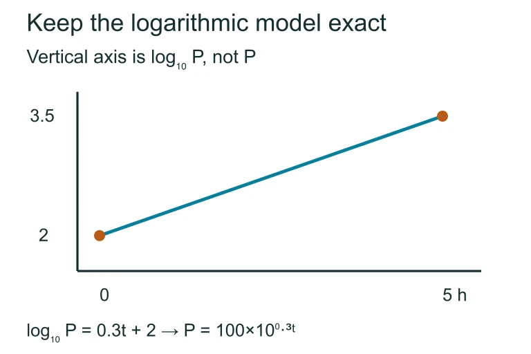 The line log₁₀P = 0.3t + 2 gives P = 100×10^(0.3t). Its hourly growth factor is about 1.995.
Semi-log vs. Log-log Plots
| Semi-log | Log-log | |
|---|---|---|
| Axes | \(\log y\) vs. \(x\) | \(\log y\) vs. \(\log x\) |
| Linearizes | Exponential models \(y = ab^{x}\) | Power models \(y = ax^{n}\) |
| Slope gives | \(\log b\) (base of exponent) | \(n\) (power/exponent) |
| Intercept gives | \(\log a\) (initial value) | \(\log a\) (coefficient) |
Checking Model Fit with Residuals
After fitting a line to the semi-log data, compute residuals: the differences between observed \(\log y\) values and the values predicted by the line.
How to Build a Semi-log Model
Example 1: Bacteria Growth
A culture starts with 50 bacteria and doubles every hour. Data after 0, 1, 2, 3, 4, and 5 hours:
| \(x\) (hours) | \(y\) (count) | \(\log y\) |
|---|---|---|
| 0 | 50 | 1.699 |
| 1 | 100 | 2.000 |
| 2 | 200 | 2.301 |
| 3 | 400 | 2.602 |
| 4 | 800 | 2.903 |
| 5 | 1600 | 3.204 |
Example 1: Finding the Model
Example 2: Radioactive Decay
A substance has a half-life of 3 days. Starting mass: 800 g. A semi-log plot of \(\log y\) vs. \(x\) (days) passes through the points \((0,\,2.903)\) and \((3,\,2.602)\).
Example 3: Natural Log Version
Some semi-log plots use \(\ln y\) instead of \(\log_{10} y\). The algebra is the same but with base \(e\):
Suppose a semi-log plot (\(\ln y\) vs. \(x\)) has slope \(k = 0.05\) and intercept \(\ln a = 6.91\). Then:
When the Semi-log Plot Curves
Common Mistakes to Avoid
Summary at a Glance
| Feature | Semi-log Plot |
|---|---|
| Axes | \(\log y\) (vertical) vs. \(x\) (horizontal) |
| Data model | \(y = ab^{x}\) (exponential) |
| Linear form | \(\log y = (\log b)x + \log a\) |
| Slope means | \(\log b\): multiplicative rate per unit \(x\) |
| Intercept means | \(\log a\): initial value (at \(x = 0\)) |
| Positive slope | Exponential growth (\(b > 1\)) |
| Negative slope | Exponential decay (\(b < 1\)) |
| Curved data | Not exponential: try another model |
Question 1 of 5
On a semi-log plot, \(\log y\) is plotted against \(x\) and the data forms a straight line. What type of function does the original data follow?
Question 2 of 5
A semi-log regression line has slope \(m = 0.477\) and y-intercept \(c = 2\). What is the exponential model?
Question 3 of 5
On a semi-log plot, the regression line has a negative slope. What does this tell you about the original data?
Question 4 of 5
Data points on a semi-log plot form a curve rather than a line. Which conclusion is most appropriate?
Question 5 of 5
A semi-log plot using \(\ln y\) vs. \(x\) has slope \(k = 0.03\) and intercept \(\ln a = 4.605\). What is the model?