01 / 21

Polynomial Functions
and Rates of Change

Explore how polynomial functions behave through average and instantaneous rates of change, and connect slopes of secant and tangent lines to real-world meaning.

AP Precalculus

What Is a Polynomial Function?

A polynomial function is a function of the form:

$$ f(x) = a_n x^n + a_{n-1} x^{n-1} + \cdots + a_1 x + a_0 $$

where \( n \) is a non-negative integer (the degree), \( a_n \neq 0 \), and each \( a_i \) is a real-number coefficient.

Degree
The highest power of \( x \) determines the polynomial's overall shape and end behavior.
Leading Coefficient
The coefficient \( a_n \) controls whether the graph opens up or down and how steeply it rises or falls.

Visualizing Polynomial Behavior

x y Cubic -3 0 3

Why Rates of Change Matter

A rate of change tells us how quickly a function's output changes relative to its input. For polynomial functions, rates of change reveal:

Where it grows
Positive rates mean the function is increasing: output rises as input increases.
Where it shrinks
Negative rates mean the function is decreasing: output falls as input increases.
Where it turns
A rate of zero marks a local extremum: a peak or valley where the function changes direction.

The Average Rate of Change

The average rate of change (AROC) of \( f \) on the interval \([a, b]\) is the slope of the secant line through the points \((a, f(a))\) and \((b, f(b))\):

$$ \text{AROC} = \frac{f(b) - f(a)}{b - a} $$

x y
\((a, f(a))\)
\((b, f(b))\)
Secant line
\(f(b)-f(a)\)
\(b - a\)

The Instantaneous Rate of Change

As the interval \([a, b]\) shrinks (i.e., \( b \to a \)), the secant line approaches the tangent line at \( x = a \). Its slope is the instantaneous rate of change:

$$ \text{IROC at } x = a = \lim_{h \to 0} \frac{f(a+h) - f(a)}{h} $$

AROC vs IROC: Key Distinction

Average ROC (AROC) Instantaneous ROC (IROC)
Interval Over \([a, b]\) At a single point \( x = a \)
Geometric meaning Slope of secant line Slope of tangent line
Formula \(\frac{f(b)-f(a)}{b-a}\) \(\lim_{h \to 0}\frac{f(a+h)-f(a)}{h}\)
What it tells you Overall behavior between two points Exact behavior at one point
AP Precalc approach Direct calculation Estimate via shrinking intervals

Rates of Change of Rates of Change

Just as we can compute the rate of change of \( f(x) \), we can compute the rate of change of the AROC itself. This reveals the function's concavity.

AROC increasing
The function is concave up: the curve bends upward, like the inside of a bowl.
AROC decreasing
The function is concave down: the curve bends downward, like the top of a hill.

How to Compute AROC: Step by Step

1
Identify the interval. Determine the two \( x \)-values \( a \) and \( b \) for your interval \([a, b]\).
2
Evaluate the function. Compute \( f(a) \) and \( f(b) \) by substituting into the polynomial.
3
Apply the formula. Calculate \(\displaystyle \frac{f(b) - f(a)}{b - a}\).
4
Interpret the result. Positive means increasing on average; negative means decreasing; zero means no net change.

Example 1: AROC of a Quadratic

Find the average rate of change of \( f(x) = x^2 - 4x + 3 \) on \([1, 4]\).

1
Evaluate: \( f(1) = 1 - 4 + 3 = \) \(0\)
2
Evaluate: \( f(4) = 16 - 16 + 3 = \) \(3\)
3
Compute AROC: \(\displaystyle \frac{f(4) - f(1)}{4 - 1} = \frac{3 - 0}{3} = \) \(1\)

Example 2: AROC of a Cubic

Find the average rate of change of \( g(x) = x^3 - 3x \) on \([-1, 2]\).

1
Evaluate: \( g(-1) = (-1)^3 - 3(-1) = -1 + 3 = \) \(2\)
2
Evaluate: \( g(2) = 8 - 6 = \) \(2\)
3
Compute AROC: \(\displaystyle \frac{g(2) - g(-1)}{2 - (-1)} = \frac{2 - 2}{3} = \) \(0\)

Example 3: Estimating the IROC

Estimate the instantaneous rate of change of \( f(x) = x^2 \) at \( x = 3 \) using shrinking intervals.

Interval AROC
\([3,\, 4]\) \(\frac{16 - 9}{1} = 7\)
\([3,\, 3.1]\) \(\frac{9.61 - 9}{0.1} = 6.1\)
\([3,\, 3.01]\) \(\frac{9.0601 - 9}{0.01} = 6.01\)
\([3,\, 3.001]\) \(\frac{9.006001 - 9}{0.001} = 6.001\)

Second Differences and Polynomial Degree

For equally spaced input values, the pattern of differences reveals the polynomial's degree:

1
Linear (degree 1): First differences are constant.
2
Quadratic (degree 2): Second differences are constant.
3
Cubic (degree 3): Third differences are constant.
4
In general, a degree-\( n \) polynomial has constant \(n\)-th differences.

Visualizing Concavity

Concave Up AROC is increasing Concave Down AROC is decreasing

Common Mistakes to Avoid

✕ Reversing the formula
Writing \(\frac{b - a}{f(b) - f(a)}\) instead of \(\frac{f(b) - f(a)}{b - a}\). Remember: output change over input change.
✕ AROC of 0 means constant
An AROC of 0 means the net change is zero, not that the function is flat. It may rise and fall within the interval.
✕ Confusing AROC with IROC
AROC is over an interval; IROC is at a point. Using a wide interval to claim you found the instantaneous rate is incorrect.

Summary: Polynomial Rates of Change

Concept What It Tells You How to Find It
AROC Average behavior over \([a,b]\) \(\frac{f(b)-f(a)}{b-a}\)
IROC Exact behavior at \(x = a\) Limit of AROC as interval shrinks
Positive ROC Function is increasing Output rises as input rises
Negative ROC Function is decreasing Output falls as input rises
Increasing AROC Concave up Second differences positive
Decreasing AROC Concave down Second differences negative

Worked practice: Practice Problems — road elevation data

Work through this original lesson problem, then reveal the solution and illustrations.

A civil engineer models the elevation (in meters) of a road profile along a 4 km stretch using a polynomial function E. Elevation data is collected at equally spaced 1 km intervals: Distance x (km): 0, 1, 2, 3, 4 Elevation E(x) (m): 120, 135, 142, 137, 116 (a) Compute the average rate of change of E over each of the four consecutive 1-km intervals. (b) Explain what the sampled rates suggest about concavity on [1,3]. Are they sufficient to prove concavity without restricting the polynomial model? (c) Compute the second differences and third differences. Based on these, what is the minimum possible degree of E? Explain. (d) The engineer states that the road profile has an interior maximum on [1,3]. Use the given elevations and continuity to justify this claim.

Show answer and explanation

Point 1 (1 pt): AROC computations. AROC on [0,1] = (135 − 120)/1 = 15; AROC on [1,2] = (142 − 135)/1 = 7; AROC on [2,3] = (137 − 142)/1 = −5; AROC on [3,4] = (116 − 137)/1 = −21. All four values must be correct. Point 2 (1 pt): The sampled slopes 7 and −5 decrease, which is consistent with concave-down behavior, but two secant slopes do not prove concavity between stations for an unrestricted polynomial. If E is restricted to the minimum-degree interpolating cubic, E(x) = 120 + (53/3)x − 2x² − (2/3)x³ and E″(x) = −4 − 4x < 0 on [1,3], so that model is concave down. Award the point for distinguishing evidence from proof and stating the model restriction for a definite conclusion. Point 3 (1 pt): Second differences = 7 − 15 = −8; −5 − 7 = −12; −21 − (−5) = −16. These are −8, −12, −16—not constant. Third differences = −12 − (−8) = −4; −16 − (−12) = −4. Third differences are constant at −4, so the minimum degree is 3 (cubic). Point 4 (1 pt): E(2) = 142 is greater than E(1) = 135 and E(3) = 137. By continuity and the extreme value theorem, E attains a maximum on [1,3], and neither endpoint can be a maximizing point. Therefore a maximum occurs in the interior. This does not prove that the global maximum on [0,4] lies there. Award the point for this argument; do not apply the intermediate value theorem to sampled average rates.
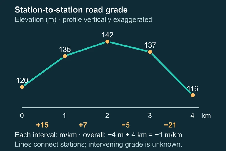
Road elevations 120,135,142,137,116 m at distances 0,1,2,3,4 km, with interval average grades 15,7,−5,−21 m/km. Between-station grade is not determined by straight connectors.
Survey endpoint changes give net average grade−1 m/km across the route without determining every slope between stations.

Question 1 of 5

What is the average rate of change of \( f(x) = 2x^2 + 1 \) on the interval \[[1, 3]\]?

Question 2 of 5

The average rate of change of a function on \([2, 5]\) is 0. Which statement must be true?

Question 3 of 5

A function has AROC values of 2, 4, 6, 8 over four consecutive equal-width intervals. What can you conclude?

Question 4 of 5

To estimate the instantaneous rate of change of \( f(x) = x^3 \) at \( x = 2 \), which approach is best?

Question 5 of 5

For a polynomial with equally spaced inputs, the second differences of the outputs are constant. What is the degree of this polynomial?