01 / 21

Function Model
Selection & Assumptions

Learn to choose the right function model for real-world data and clearly articulate the assumptions behind your choice.

AP Precalculus

What Is a Function Model?

A function model is a mathematical function chosen to represent a real-world relationship. We write \( y = f(x) \) where the formula for \( f \) is selected to approximate observed data or a described scenario.

Linear
\( f(x) = mx + b \): constant rate of change
Quadratic
\( f(x) = ax^2 + bx + c \): changing rate of change
Exponential
\( f(x) = ab^x \): proportional growth or decay

Why Model Selection Matters

Time Population Linear Exponential

The linear model predicts a steady decrease, while the exponential model predicts a decelerating decrease. Both fit the current data, but their long-term predictions diverge dramatically.

What Are Model Assumptions?

Every model carries implicit assumptions about the behavior of the quantities involved. Selecting a model means claiming these assumptions are reasonable for the context.

1
Linear assumption: The rate of change \( \frac{\Delta y}{\Delta x} \) is constant across the domain.
2
Exponential assumption: The output changes by a constant ratio over equal input intervals: \( \frac{f(x+d)}{f(x)} = r \).
3
Quadratic assumption: The rate of change itself changes at a constant rate: the second differences are equal.

The Selection Principle

Observe Data Check Pattern (diffs / ratios) Select Model Articulate Assumptions

This four-step process ensures your model is justified by evidence and your assumptions are transparent and testable.

Diagnostic Tests for Each Model

Linear Quadratic Exponential
Test First differences constant Second differences constant Consecutive ratios constant
Formula \( \Delta y = c \) \( \Delta^2 y = c \) \( \frac{y_{n+1}}{y_n} = r \)
Assumption Constant rate Rate changes linearly Proportional growth

Linear vs. Exponential

0 1 2 3 4 5 Linear Exponential +35 each ×1.5 each
Linear
Constant additive change: \( f(x+1) = f(x) + d \). Assumption: the quantity grows by a fixed amount per unit.
Exponential
Constant multiplicative change: \( f(x+1) = f(x) \cdot r \). Assumption: the quantity grows by a fixed percentage per unit.

How to Apply the Process

1
Organize the data. Ensure inputs are equally spaced. If not, compute average rates over each interval.
2
Compute first differences \( \Delta y = y_{n+1} - y_n \). If approximately constant: linear.
3
Compute consecutive ratios \( r = y_{n+1}/y_n \). If approximately constant: exponential.
4
Compute second differences \( \Delta^2 y \). If approximately constant: quadratic.
5
State your assumption explicitly: "We assume [quantity] changes at a constant [rate/ratio/second rate] because..."

Example 1: Water Tank

A tank drains at a constant rate. Data recorded every minute:

Time (min) 0 1 2 3 4
Volume (L) 200 175 150 125 100
\( \Delta y \) −25 −25 −25 −25

Example 2: Bacteria Growth

A colony is measured every hour:

Hour 0 1 2 3 4
Count 500 750 1125 1688 2531
\( \Delta y \) 250 375 563 843
\( y_{n+1}/y_n \) 1.50 1.50 1.50 1.50

Example 3: Projectile Height

A ball is launched upward. Height recorded each second:

Time (s) 0 1 2 3 4
Height (m) 0 35 60 75 80
\( \Delta y \) 35 25 15 5
\( \Delta^2 y \) −10 −10 −10

Beyond the Big Three: Other Models

Logarithmic
\( f(x) = a + b\ln x \). Growth that decelerates over time. Assumption: diminishing returns as input increases.
Logistic
\( f(x) = \frac{L}{1 + ce^{-kx}} \). Exponential start, then levels off to carrying capacity \( L \). Assumption: growth is constrained by limited resources.
x L Logarithmic Logistic

Writing Assumption Statements

On the AP exam, you must clearly articulate why a model is appropriate. Use this sentence framework:

✓
Good: "An exponential model is appropriate because the consecutive ratios are approximately constant at 1.5, implying the bacteria population grows by 50% each hour."
✕
Weak: "I chose exponential because it looks like the graph curves up." This does not reference the data pattern or the real-world meaning.

When Models Break Down

Every model has a domain of validity. Outside this domain, the assumption fails and predictions become unreliable.

Linear
Predicts negative volume when a tank is empty. Breaks when \(V(t) < 0\).
Exponential
Predicts infinite population. Breaks when resources are limited.
Quadratic
Predicts height going to \( -\infty \). Breaks once the object hits the ground.

Common Mistakes

✕ Picking by Shape
Choosing a model because "the graph curves up" without computing differences or ratios from the data.
✕ Ignoring Context
Selecting exponential for a population with known resource limits, when logistic is more appropriate.
✕ Unstated Assumptions
Writing the equation without explaining why the model fits: what real-world condition makes the pattern hold?

Model Summary Table

Property Linear Quadratic Exponential Logarithmic
General Form \( mx + b \) \( ax^2 + bx + c \) \( ab^x \) \( a + b\ln x \)
Key Test \( \Delta y \text{ const} \) \( \Delta^2 y \text{ const} \) \( \text{Ratios const} \) \( \text{Rate} \propto \frac{1}{x} \)
End Behavior \( \pm\infty \) \( \pm\infty \) \( 0 \) or \( \infty \) \( \infty \) (slowly)
Assumption Constant rate Rate changes linearly Proportional change Diminishing returns

Worked Example — Selecting and Justifying a Model

A biologist records the concentration of a nutrient (mg/L) in a lake at equally spaced weekly intervals. The data are shown below. Determine an appropriate function model and articulate the assumptions that support your choice. Week (t) | Concentration C(t) 0 | 2.0 1 | 5.0 2 | 8.0 3 | 9.5 4 | 10.0 5 | 10.3 6 | 10.4 Selecting a Model for Nutrient Concentration Step 1 — Examine End Behavior The concentration increases from 2.0 to 10.4 mg/L, while the increments decrease from 3.0 to 0.1. This observed slowing is consistent with leveling, but the finite observations do not establish an asymptote. A rational function is one candidate if a finite limiting concentration is independently justified. Candidate only: rational model with an assumed horizontal asymptote. Step 2 — Compute First Differences (Verification) First differences are 3.0, 3.0, 1.5, 0.5, 0.3, 0.1; second differences are 0, −1.5, −1.0, −0.2, −0.2. Their variation rules out exact linear and exact quadratic interpolation of every point. It does not exclude all higher-degree polynomials, nor prove long-run leveling. No exact linear or quadratic fit; finite data do not determine end behavior. Step 3 — Propose a Specific Rational Form Assume, as a candidate rather than a measured fact, that the limiting concentration is 10.5 mg/L. Explore C(t) = (at + b)/(t + c). Here, the degree of the numerator equals the degree of the denominator (both degree 1), so the horizontal asymptote is y = a/1 = a. We estimate a ≈ 10.5. Using C(0) = 2 gives b/c = 2, and using C(1) = 5 gives (a + b)/(1 + c) = 5. Solving this system with a = 10.5 yields approximately: C(t) = (10.5t + 2·c)/(t + c). From C(0) = 2: b = 2c. From C(1) = 5: (10.5 + 2c)/(1 + c) = 5, so 10.5 + 2c = 5 + 5c, giving c = 11/6 ≈ 1.833 and b ≈ 3.667. Candidate: C(t) = (10.5t + 11/3)/(t + 11/6). It matches t = 0,1 but predicts C(2) ≈ 6.435 and C(6) ≈ 8.511, below observed 8.0 and 10.4. It is not validated by the full series. Step 4 — Articulate Assumptions This candidate assumes continuous concentration for t ≥ 0, a finite limit of 10.5 mg/L, and a diminishing rate of increase. These are modeling assumptions, not consequences proved by the seven observations. The substantial underprediction at weeks 2 and 6 shows that fitting the first two points is insufficient. A better-supported model would require further fitting and validation before prediction. Assumptions stated; the candidate fails to fit the full series closely.
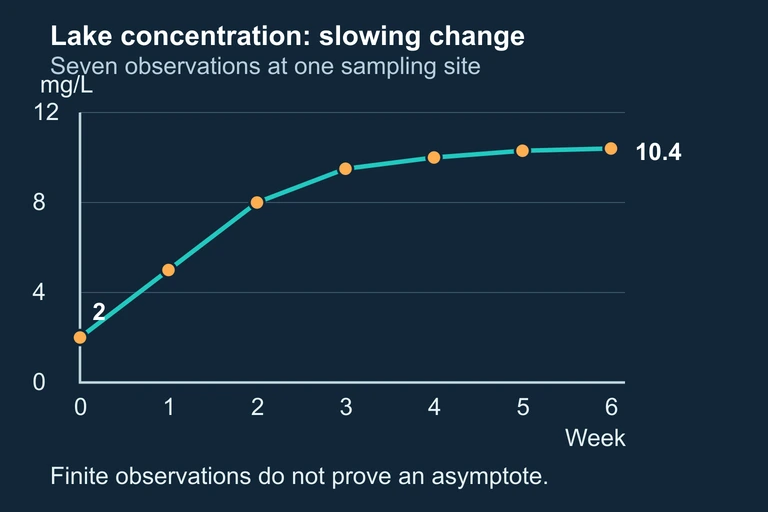
Seven weekly observed nutrient concentrations: 2,5,8,9.5,10,10.3,10.4. Finite data show slowing but do not prove an asymptote.
Seven observed lake concentrations suggest leveling within the observed window but cannot establish a unique horizontal asymptote.

Question 1 of 5

A car's value decreases each year. After year 1 it is worth \$20,000, year 2: \$16,000, year 3: \$12,800, year 4: \$10,240. Which model is most appropriate?

Question 2 of 5

If a linear model \( f(x) = 3x + 10 \) is chosen for a dataset, which assumption is being made?

Question 3 of 5

Data: \( x \): 0, 1, 2, 3, 4. \( y \): 5, 12, 23, 38, 57. The first differences are 7, 11, 15, 19. What type of model is most appropriate?

Question 4 of 5

An exponential model \( P(t) = 100 \cdot 2^t \) is used for a bacteria population. Which statement best articulates the key assumption?

Question 5 of 5

A student writes: "I chose exponential because the graph goes up fast." Which correction would most improve this justification?