Function Model
Construction & Application
Learn to build mathematical models from data and context, selecting the right function type to represent real-world relationships.
What Is a Function Model?
A function model is a mathematical function chosen to describe a real-world relationship between quantities. We use data, context clues, and known function behaviors to select and build these models.
The Model-Building Cycle
Why Do Models Matter?
Core Function Families
Constant rate of change
Changing rate of change (linear)
Constant proportional change
Rapid then slowing growth
Signature Behaviors
Linear vs. Exponential
| Linear | Exponential | |
|---|---|---|
| General Form | \( f(x) = mx + b \) | \( f(x) = a \cdot b^x \) |
| Rate of Change | Constant | Proportional to value |
| Data Test | Equal \(\Delta y\) over equal \(\Delta x\) | Equal ratio \(\frac{y_2}{y_1}\) over equal \(\Delta x\) |
| Long-term Behavior | Grows without bound, steadily | Grows without bound, accelerating |
Identifying the Right Model
Step-by-Step Model Construction
Follow the salt through a working mixing rig
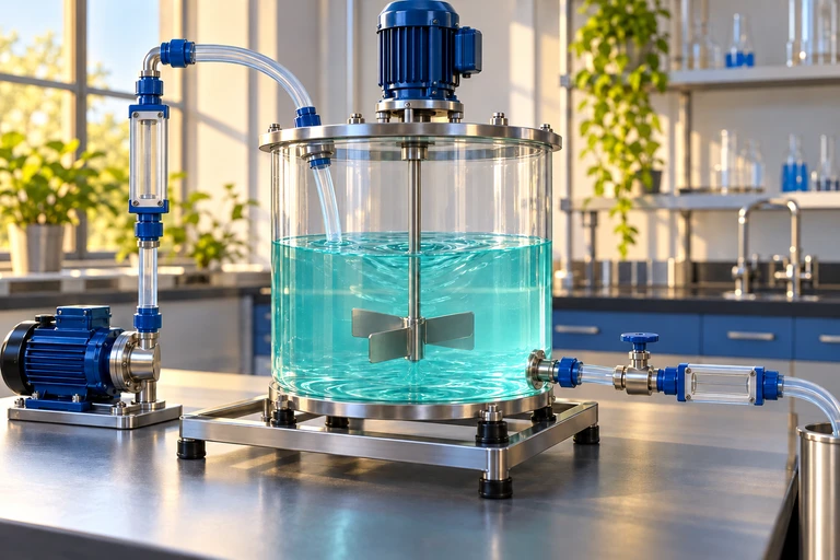 With the outlet closed, salt mass is 6t g and water volume is 50 + 2t L. Their ratio C(t) = 3t/(25 + t) g/L increases toward the incoming concentration of 3 g/L.
Filling-only concentration model
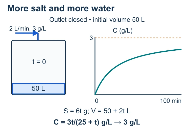 With the outlet closed, salt mass is 6t g and water volume is 50 + 2t L. Their ratio C(t) = 3t/(25 + t) g/L increases toward the incoming concentration of 3 g/L.
Example 1: Linear Model
A water tank drains at a steady rate. At \( t = 0 \) hours it holds 200 gallons, and at \( t = 5 \) hours it holds 75 gallons. Build a model for \(W(t)\).
Example 1: Graph
Example 2: Exponential Model
A bacteria culture starts with 500 cells and doubles every 3 hours. Build a model for the population \(P(t)\).
Example 2: Graph
Example 3: Quadratic from Data
A ball is launched upward. Its height \(h\) (meters) at time \(t\) (seconds) is recorded:
| \( t \) | 0 | 1 | 2 | 3 | 4 |
|---|---|---|---|---|---|
| \( h(t) \) | 2 | 27 | 42 | 47 | 42 |
| \( \Delta h \) | 25 | 15 | 5 | -5 | |
| \( \Delta^2 h \) | -10 | -10 | -10 |
Common Mistakes
Summary of Function Models
| Model | Form | Key Signal | Context Clue |
|---|---|---|---|
| Linear | \( mx + b \) | Constant \( \Delta y \) | "per year," "each month" |
| Quadratic | \( ax^2 + bx + c \) | Constant \( \Delta^2 y \) | "projectile," "area" |
| Exponential | \( a \cdot b^x \) | Constant ratio | "doubles," "half-life" |
| Logarithmic | \( a + b\ln(x) \) | Fast then slow growth | "diminishing returns" |
Question 1 of 5
A dataset has outputs 10, 20, 40, 80, 160 for equally spaced inputs. Which function type best models this data?
Question 2 of 5
A car depreciates from $20,000 by 15% each year. Which model represents its value \(V(t)\) after \(t\) years?
Question 3 of 5
The second differences of a data set are approximately constant at 6. What is the leading coefficient \(a\) in the quadratic model \(f(x) = ax^2 + bx + c\)?
Question 4 of 5
An exponential function passes through \( (0, 4) \) and \( (2, 36) \). What is the value of \(b\) in \(f(x) = a \cdot b^x\)?
Question 5 of 5
A linear model gives \(f(10) = 50\) and \(f(15) = 75\). What is \(f(20)\)?