Competing Function
Model Validation
Learn to choose the best-fit function model by analyzing residuals, comparing predicted vs. observed values, and evaluating goodness of fit.
What Is Model Validation?
When we fit a function to data, we need to check: how well does the model actually represent the data? Model validation is the process of testing a proposed function against observed values to determine if it is a reliable predictor.
Why Competing Models?
Real data rarely tells you which function type to use. The same dataset might plausibly be modeled by a linear, quadratic, or exponential function. We compare competing models to find the one that best captures the underlying behavior.
The Residual: Your Validation Tool
A residual measures the vertical distance between a data point and the model's prediction. Positive residuals mean the model underestimates; negative residuals mean it overestimates.
A cell culture where more cells create more growth events

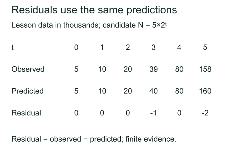
For the six observations 5, 10, 20, 39, 80, and 158 thousand, the model N = 5×2^t gives residuals 0, 0, 0, −1, 0, and −2 thousand.Competing model validation data
For the six observations 5, 10, 20, 39, 80, and 158 thousand, the model N = 5×2^t gives residuals 0, 0, 0, −1, 0, and −2 thousand.Residual Plots Reveal Model Fit
A residual plot graphs residuals vs. \( x \). The pattern tells you whether your model captures the data's structure:
The SSR Criterion
The SSR quantifies total model error. For competing models fit to the same data, the model with the smaller SSR fits better. We square residuals so positive and negative errors don't cancel out.
Measuring Fit with \( R^2 \)
\( R^2 \) tells you what fraction of the data's variability the model explains. It ranges from 0 (no explanatory power) to 1 (perfect fit). When comparing models: higher \( R^2 \) = better fit.
Overfitting vs. Underfitting
A model with more parameters will always have a higher \( R^2 \) on the training data, but it may be capturing noise rather than the true pattern. The best model balances accuracy with simplicity.
How to Validate Competing Models
Example 1: Linear vs. Quadratic
A scientist measures the height (cm) of a plant over 6 weeks. Two models are proposed:
Example 1: Residual Comparison
| Week | Observed | Linear Resid. | Quadratic Resid. |
|---|---|---|---|
| 1 | 5 | 0 | +1.8 |
| 2 | 7 | -1 | +1.1 |
| 3 | 11 | 0 | +1.4 |
| 4 | 16 | +2 | +1.7 |
| 5 | 22 | +5 | +2.0 |
| 6 | 30 | +10 | +3.3 |
Example 2: Exponential vs. Linear
A bacteria colony doubles roughly every hour. Data: \((0,\,50)\), \((1,\,98)\), \((2,\,205)\), \((3,\,410)\), \((4,\,800)\). Two models:
Example 2: Verdict
| Hour | Observed | Linear Pred. | Exp. Pred. |
|---|---|---|---|
| 0 | 50 | -50 | 50 |
| 1 | 98 | 135 | 100 |
| 2 | 205 | 320 | 200 |
| 3 | 410 | 505 | 400 |
| 4 | 800 | 690 | 800 |
Example 3: Three-Way Comparison
Revenue data (\$M) for a startup over 5 years: \((1,\,12)\), \((2,\,28)\), \((3,\,50)\), \((4,\,79)\), \((5,\,115)\). Which model fits best?
| Model | Equation | SSR | \( R^2 \) |
|---|---|---|---|
| Linear | \( 25.3x - 15.1 \) | 67.5 | 0.990 |
| Quadratic | \( 4.5x^2 + 0.8x + 7.2 \) | 16.6 | 0.998 |
| Exponential | \( 7.32 \cdot 1.74^x \) | 311.5 | 0.954 |
Common Mistakes to Avoid
Summary: Validation Criteria
| Criterion | Good Sign | Warning Sign |
|---|---|---|
| Residual Plot | Random scatter | Curved or fanning pattern |
| SSR | Small relative to SST | Large or much worse than rival |
| \( R^2 \) | Close to 1 | Low or only slightly better with added complexity |
| Model Predictions | Physically plausible | Negative values, divergence outside domain |
| Simplicity | Fewest parameters needed | Over-parameterized: fits noise |
Worked Example: Choosing Between Exponential and Quadratic
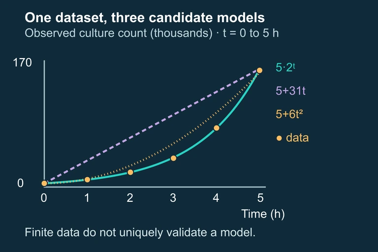
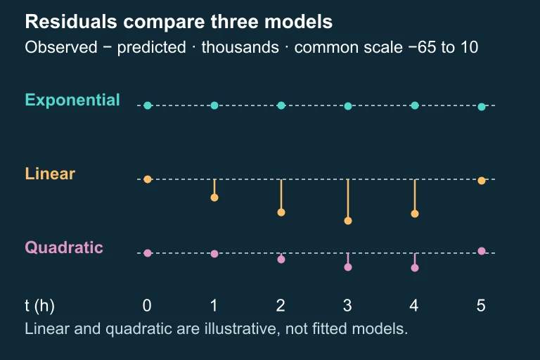
Consider the following data set collected from a biological experiment measuring the number of bacteria (in thousands) in a culture over equally spaced time intervals. t (hours) | 0 | 1 | 2 | 3 | 4 | 5 N(t) | 5 | 10 | 20 | 39 | 80 | 158 Step 1 — Compute First Differences Δy: 10 − 5 = 5, 20 − 10 = 10, 39 − 20 = 19, 80 − 39 = 41, 158 − 80 = 78. The first differences are 5, 10, 19, 41, 78—clearly not constant, so no linear function passes exactly through all six observations. No exact linear fit — first differences vary. Step 2 — Compute Consecutive Ratios r: 10/5 = 2.00, 20/10 = 2.00, 39/20 = 1.95, 80/39 ≈ 2.05, 158/80 ≈ 1.975. All ratios are approximately 2.0, suggesting an exponential model with base b ≈ 2. Ratios ≈ 2.0 — strong exponential signal. Step 3 — Check Second Differences (Competing Test) Δ²y: 10 − 5 = 5, 19 − 10 = 9, 41 − 19 = 22, 78 − 41 = 37. The second differences are 5, 9, 22, 37—these are not constant, so no quadratic function passes exactly through all six observations. No exact quadratic fit — second differences vary. Step 4 — Propose an Exponential Model and Examine Residuals Using N(0) = 5 and the near-constant ratio 2, propose N(t) = 5·2ᵗ. Predictions are 5, 10, 20, 40, 80, 160, with residuals 0, 0, 0, −1, 0, −2. This candidate fits closely over the observed interval, but six small residuals do not establish uniqueness, a patternless error process, or future accuracy. The supplemental curves 5 + 31t and 5 + 6t² are illustrative comparators, not least-squares fits. N(t) = 5·2ᵗ fits closely here; further validation is needed. VALIDATION STRATEGY
Question 1 of 5
A residual plot for a linear model shows a clear U-shaped curve. What does this suggest?
Question 2 of 5
Model A has \( R^2 = 0.92 \) and Model B has \( R^2 = 0.97 \). Model A uses 2 parameters; Model B uses 5. Which statement is most accurate?
Question 3 of 5
For data points \((1,\,10)\), \((2,\,22)\), \((3,\,35)\), a model predicts \(\hat{y} = 11x - 2\). What is the residual at \( x = 2 \)?
Question 4 of 5
An exponential model \( \hat{y} = 5 \cdot 1.5^x \) predicts a population. At \( x = 0 \), the observed value is 5. What is the SSR contribution from this point?
Question 5 of 5
Which is the best reason to reject a model even if it has a high \( R^2 \)?