01 / 21

Change in Linear and
Exponential Functions

Understand how constant rate of change differs from proportional rate of change, and learn to identify, compare, and apply both function types.

AP Precalculus

What Is Change in a Function?

When we study functions, we care about how output values change as input values change. The way a function's output responds to equal steps in input reveals its fundamental nature.

Input Change
A consistent step in \(x\): for example, moving from \(x\) to \(x+1\)
Output Change
How \(f(x)\) responds: does it add a constant or multiply by a constant?

Linear Functions: Constant Rate of Change

A linear function has the form \(f(x) = mx + b\). Over equal intervals of the input, the output changes by a constant amount \(m\), called the slope or rate of change.

x y +2 +2 +2 0 1 2 3 4 5 \(f(x) = 2x + 1\)

Exponential Functions: Proportional Change

An exponential function has the form \(g(x) = a \cdot b^x\). Over equal intervals, the output is multiplied by a constant factor \(b\), called the base or growth/decay factor.

x y 0 1 2 3 4 5 \(\times 2\) \(\times 2\) \(\times 2\) \(\times 2\) \(g(x) = 2^x\)

The Key Formulas

Linear Function
\(f(x) = mx + b\)

Average rate of change over \([a, b]\):
\(\displaystyle \frac{f(b) - f(a)}{b - a} = m\)

Always equals the slope \(m\).
Exponential Function
\(g(x) = a \cdot b^x\)

Over equal intervals of length 1:
\(\displaystyle \frac{g(x+1)}{g(x)} = b\)

Output is multiplied by \(b\).

Average Rate of Change

For any function \(f\), the average rate of change over \([a, b]\) is:

1
Linear: AROC is the same over every interval. It equals the slope \(m\).
2
Exponential (growth, \(b > 1\)): AROC increases as \(x\) increases.
3
Exponential (decay, \(0 < b < 1\)): AROC approaches zero as \(x\) increases.

Adding vs Multiplying

Linear Exponential
Form \(f(x) = mx + b\) \(g(x) = a \cdot b^x\)
Output pattern Add \(m\) each step Multiply by \(b\) each step
First differences Constant Not constant
Consecutive ratios Not constant Constant
AROC behavior Same everywhere Increasing or decreasing
Graph shape Straight line Curve (concave up for \(a > 0\))

Identifying from a Table

Given equally spaced \(x\)-values, check two things:

1
Compute first differences: \(f(x_{n+1}) - f(x_n)\). If all are equal, it is linear.
2
Compute consecutive ratios: \(\frac{f(x_{n+1})}{f(x_n)}\). If all are equal, it is exponential.
3
If neither is constant, the function is neither linear nor exponential.

How to Apply the Concepts

1
Identify the model: Is the function given as a formula, table, or graph?
2
Check for constant differences (linear) or constant ratios (exponential).
3
Extract parameters: For linear, find \(m\) and \(b\). For exponential, find \(a\) and \(b\).
4
Compute AROC over the requested interval using \(\frac{f(b) - f(a)}{b - a}\).
5
Interpret the result: Include units and context. Is the rate increasing, decreasing, or constant?

Example 1: Linear Table

\(x\) 01234
\(f(x)\) 58111417

Example 2: Exponential Table

\(x\) 01234
\(g(x)\) 36122448

Example 3: Comparing AROC

Compare the average rate of change of \(f(x) = 3x + 5\) and \(g(x) = 3 \cdot 2^x\) over \([1, 3]\).

Linear \(f\)
\(\displaystyle \frac{f(3) - f(1)}{3 - 1} = \frac{14 - 8}{2} = 3\)

AROC = 3 (same as always)
Exponential \(g\)
\(\displaystyle \frac{g(3) - g(1)}{3 - 1} = \frac{24 - 6}{2} = 9\)

AROC = 9 (increasing)

Linear vs Exponential Growth

x y 0 1 2 3 4 5 6 0 10 20 30 40 50 Same start \(f(x) = 5x + 3\) \(g(x) = 3 \cdot 2^x\)

Exponential Decay: \(0 < b < 1\)

When the base \(b\) is between 0 and 1, the function decreases. The output is multiplied by a fraction each step, so it shrinks toward zero but never reaches it.

x y 64 32 16 8 4 \(\times\frac{1}{2}\) \(\times\frac{1}{2}\) \(\times\frac{1}{2}\) \(y=0\) \(h(x) = 64 \cdot \left(\tfrac{1}{2}\right)^x\)

Concavity and Changing AROC

For exponential functions, the AROC itself changes. This connects to concavity:

Growth (\(b > 1\))
AROC increases over successive intervals. The graph is concave up: the curve bends upward.
Decay (\(0 < b < 1\))
AROC becomes less negative (approaches 0). The graph is also concave up: the curve bends upward from below.

Common Mistakes

✕ Confusing Differences and Ratios
Checking differences for an exponential function (or ratios for a linear function). Linear: check differences. Exponential: check ratios.
✕ Unequal Input Spacing
Applying the first-differences test when the \(x\)-values are not equally spaced. This gives false results.
✕ Thinking AROC is Constant for Exponentials
The AROC of an exponential changes with each interval. Only linear functions have constant AROC.

Worked Example

Determining and Comparing Linear and Exponential Models from Data Step 1 — Read the Problem A biologist records the mass (in grams) of a bacterial colony at equally spaced time intervals: t = 0, 1, 2, 3, 4 (hours). The data are M(0) = 5, M(1) = 10, M(2) = 20, M(3) = 40, M(4) = 80. Meanwhile, a nutrient supply N(t) is added linearly: N(0) = 5, N(1) = 15, N(2) = 25, N(3) = 35, N(4) = 45. (a) Confirm M is exponential and N is linear. (b) Write explicit formulas. (c) Find when the average rate of change of M first exceeds 50 g/hr over a unit interval. Step 2 — Test M(t) for Exponential Behavior Compute consecutive ratios: M(1)/M(0) = 10/5 = 2, M(2)/M(1) = 20/10 = 2, M(3)/M(2) = 40/20 = 2, M(4)/M(3) = 80/40 = 2. All ratios equal 2, confirming M(t) is exponential with base b = 2 and initial value a = 5. M(t) = 5 · 2ᵗ Step 3 — Test N(t) for Linear Behavior Compute first differences: N(1) − N(0) = 10, N(2) − N(1) = 10, N(3) − N(2) = 10, N(4) − N(3) = 10. All differences equal 10, confirming N(t) is linear with slope m = 10 and initial value b = 5. N(t) = 5 + 10t Step 4 — Average Rate of Change of M over Unit Intervals The average rate of change on [t, t+1] is M(t+1) − M(t). Compute: [0,1]: 10 − 5 = 5; [1,2]: 20 − 10 = 10; [2,3]: 40 − 20 = 20; [3,4]: 80 − 40 = 40. These rates themselves double each step (factor of b = 2), confirming the rate of change of an exponential is also exponential. Continuing: on [4,5] the rate would be 5 · 2⁴ = 80; on [5,6] it would be 5 · 2⁵ = 160. Step 5 — Identify the Interval Where Rate Exceeds 50 The average rate of change on [t, t+1] is M(t+1) − M(t) = 5 · 2ᵗ⁺¹ − 5 · 2ᵗ = 5 · 2ᵗ(2 − 1) = 5 · 2ᵗ. Set 5 · 2ᵗ > 50, giving 2ᵗ > 10, so t > log₂(10) ≈ 3.32. Since we need t to be an integer (starting a unit interval), the first such interval is [4, 5], where the rate of change is 5 · 2⁴ = 80 g/hr. The average rate of change of M first exceeds 50 g/hr on the interval [4, 5].
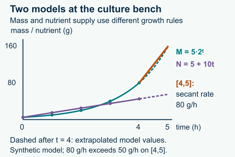
Exponential mass B(t)=5·2^t and linear nutrient model 5+10t, with extrapolation after 4 hours distinguished. Average mass change from hour 4 to 5 is 80 g/h.
The selected culture-mass model doubles hourly while nutrient supply increases linearly; these are stipulated models rather than unique conclusions from finite samples.

Question 1 of 5

A function \(f\) has the property that over equal-length input intervals, the output values have a constant ratio. What type of function is \(f\)?

Question 2 of 5

Given the table below, what is the average rate of change of \(f\) over \([1, 4]\)?

\(x\) 1234
\(f(x)\) 261854

Question 3 of 5

For the function \(g(x) = 5 \cdot 3^x\), what is the value of \(\displaystyle \frac{g(x+1)}{g(x)}\)?

Question 4 of 5

A population doubles every year, starting at 100. Which function models this, and what is its average rate of change over \([0, 3]\)?

Question 5 of 5

The graph of an exponential function \(f(x) = a \cdot b^x\) with \(a > 0\) and \(b > 1\) is always: