

SECTION 1
Historical Context & Motivation
The study of sinusoidal functions originates in humanity's oldest scientific endeavor: astronomy. Ancient Babylonian and Greek astronomers recognized that celestial positions repeat in predictable cycles, and they sought mathematical descriptions for these patterns. The Greek mathematician Hipparchus constructed the first known table of chords around 150 BCE, effectively tabulating values analogous to modern sine values. This trigonometric machinery was refined over centuries by Indian, Islamic, and European scholars until it became the foundation for modeling any phenomenon that oscillates—sound waves, tides, alternating current, and biological rhythms alike.
~150 BCE • Hipparchus' Chord Tables
~500 CE • Indian Sine Function
1748 • Euler's Analytic Framework
1822 • Fourier's Theorem
Fourier's insight raises a powerful question: if every periodic phenomenon can be expressed in terms of sinusoids, then mastering the behavior of a single sinusoidal function—its amplitude, period, phase shift, and vertical shift—gives you the toolkit to analyze virtually any repeating pattern in nature. That is precisely the goal of this lesson.
SECTION 2
Core Principles & Definitions
A sinusoidal function is any function that can be written as a transformed sine or cosine. Because cosine is simply a phase-shifted sine (cos x = sin(x + π/2)), every sinusoidal function can be expressed in either form. The AP Precalculus framework asks you to identify four key parameters that control the shape and position of the graph, and to move fluently between graphical, algebraic, and contextual representations.
Amplitude |a|
Period T = 2π / |b|
Phase Shift −c / b
Midline y = d
SECTION 3
Visual Explanation — Anatomy of a Sinusoidal Curve
Observe that the sinusoidal curve is perfectly symmetric about its midline: the distance from the midline to the maximum equals the distance from the midline to the minimum, and both equal |a|. A single period contains exactly one maximum, one minimum, and two midline crossings (one ascending, one descending). On the AP exam, you will frequently be given a partial graph and asked to extract these four parameters, so develop the habit of first locating the midline, then measuring amplitude and period, and finally noting any horizontal shift.
SECTION 4
Mathematical Framework
The general sinusoidal model used throughout AP Precalculus takes two equivalent forms. Understanding both is essential because certain contexts favor sine while others favor cosine, and the exam expects fluency in either representation.
GENERAL SINE FORM
a = amplitude (if a > 0, standard orientation; if a < 0, reflected over midline). b = frequency parameter; period T = 2π / |b|. c = phase shift (positive → right, negative → left). d = vertical shift (midline y = d).
GENERAL COSINE FORM
All parameters have the same meaning. The only difference is the starting behavior: cosine begins at a maximum (when a > 0) rather than at the midline.
PARAMETER EXTRACTION FROM DATA
Given a table or graph, compute the midline d first, then the amplitude |a|. Identify the period T as the horizontal distance between two consecutive maxima (or minima), and solve for b. Determine c by finding where the function reaches a known reference point (e.g., a maximum for cosine form).
A critical relationship that the AP course emphasizes is between the concavity of a sinusoidal function and its position relative to the midline. When the function value is above the midline, the graph is concave down (curving toward the midline), and when below the midline, it is concave up. Points of inflection occur exactly at midline crossings. This connection between position and concavity is a recurring theme in AP Precalculus free-response questions, where students must justify the behavior of rate of change.
SECTION 5
Transformations & Classification of Sinusoidal Graphs
Every sinusoidal function is obtained from the parent function y = sin x (or y = cos x) through a sequence of transformations. The AP framework treats these as compositions of vertical and horizontal stretches, reflections, and translations. The order in which you apply them matters: work inside-out, handling horizontal transformations (b and c) first, then vertical transformations (a and d).
| Transformation | Parameter Changed | Effect on Graph |
|---|---|---|
| Vertical stretch / compress | |a| > 1 or |a| < 1 | Taller or shorter waves; amplitude changes |
| Horizontal stretch / compress | |b| > 1 or |b| < 1 | Shorter or longer period; cycles speed up or slow down |
| Reflection over midline | a < 0 | Maxima become minima and vice versa |
| Horizontal translation | c ≠ 0 | Entire graph shifts left (c < 0) or right (c > 0) |
| Vertical translation | d ≠ 0 | Midline moves up or down; range shifts accordingly |
Summary of sinusoidal transformations
SECTION 6
Worked Example — Writing a Sinusoidal Model
Suppose the average monthly temperature in a city ranges from a low of 28 °F in January (month 1) to a high of 82 °F in July (month 7). We are asked to write a sinusoidal function T(m) that models the temperature as a function of the month number m.
Worked example
- 1
Step 1 — Find the Midline
The midline is the average of the maximum and minimum temperatures: d = (82 + 28) / 2 = 110 / 2.d = 55 °F - 2
Step 2 — Find the Amplitude
The amplitude is half the range: |a| = (82 − 28) / 2 = 54 / 2.|a| = 27 °F - 3
Step 3 — Determine the Period and b
Temperature cycles once per year (12 months), so T = 12. Then b = 2π / T = 2π / 12 = π / 6.b = π / 6 - 4
Step 4 — Choose Cosine and Find Phase Shift
Using cosine is natural because cosine starts at a maximum. The maximum temperature occurs at month 7, so we need cos(b(m − c)) = 1 when m = 7. This gives c = 7.c = 7 - 5
Step 5 — Assemble the Model
Combining all parameters: T(m) = 27 cos(π/6 (m − 7)) + 55. We can verify: T(7) = 27 cos(0) + 55 = 27 + 55 = 82 ✓ and T(1) = 27 cos(π/6 × (−6)) + 55 = 27 cos(−π) + 55 = 27(−1) + 55 = 28 ✓.T(m) = 27 cos(π/6 (m − 7)) + 55
 The harbor scene introduces periodic change; the accompanying graph models annual temperature. The temperature model has minimum 28 °F at month 1 and maximum 82 °F at month 7. Its midline is 55 °F, amplitude 27 °F, and period 12 months.
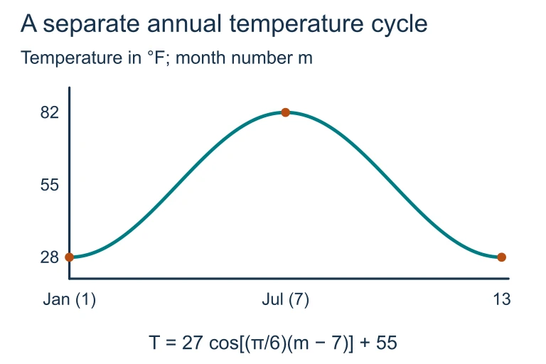 The harbor scene introduces periodic change; the accompanying graph models annual temperature. The temperature model has minimum 28 °F at month 1 and maximum 82 °F at month 7. Its midline is 55 °F, amplitude 27 °F, and period 12 months.
SECTION 7
Sine vs. Cosine — When to Use Which
Since cosine is simply sine shifted left by π/2, the choice between the two is ultimately a matter of convenience. However, strategic selection can simplify your algebra considerably. The table below summarizes common scenarios and the preferred form for each.
| Scenario | Preferred Form | Reason |
|---|---|---|
| Data starts at a maximum | Cosine (a > 0) | Cosine's parent starts at its max; phase shift equals the x-coordinate of the max. |
| Data starts at a minimum | Cosine (a < 0) or −cos | Negating cosine flips the max to a min at x = c. |
| Data starts at the midline, increasing | Sine (a > 0) | Sine's parent crosses the midline going up at x = 0. |
| Data starts at the midline, decreasing | Sine (a < 0) or −sin | Negating sine starts at the midline going down. |
| Calculator regression | Sine (standard form) | Most graphing calculators output sinusoidal regression as a sin(bx + c) + d. |
Quick-reference guide for choosing sine or cosine
SECTION 8
Connections to Calculus & Advanced Analysis
Sinusoidal functions occupy a privileged position in mathematics because they are eigenfunctions of differentiation: differentiating sine yields cosine (a phase shift), and differentiating again returns −sin. This self-reproducing property makes sinusoids indispensable in differential equations and signal processing. The table below previews how your AP Precalculus sinusoidal toolkit extends into calculus.
| AP Precalculus Concept | Calculus / Advanced Extension |
|---|---|
| Amplitude & midline | Determine maximum rate of change (derivative amplitude = a × b) |
| Period T = 2π/|b| | Frequency f = 1/T; angular frequency ω = 2πf = |b| (ubiquitous in physics) |
| Concavity & midline crossing | Second derivative test: inflection points occur at midline crossings |
| Phase shift c | In Fourier analysis, phase encodes how component waves align to form complex signals |
| Sinusoidal regression | Leads to Fourier series: decomposing any periodic function into infinite sums of sinusoids |
From AP Precalculus to Calculus and beyond
While you will not be tested on derivatives or Fourier series in AP Precalculus, understanding that sinusoidal functions are the fundamental building blocks of all periodic analysis gives valuable perspective. Every time you write f(x) = a sin(b(x − c)) + d, you are constructing one term of a potentially infinite sum that can approximate even a square wave or a heartbeat.
SECTION 9
Practice Problems
Question 1: CONCEPTUAL
- A. Amplitude = 12, Midline y = 5
- B. Amplitude = 6, Midline y = 4
- C. Amplitude = 6, Midline y = 5
- D. Amplitude = 10, Midline y = 4
- E. Amplitude = 5, Midline y = 6
Show answer (B)
Question 2: BASIC CALCULATION
- A. 4π
- B. 2π
- C. π/2
- D. π/4
- E. π
Show answer (C)
Question 3: INTERMEDIATE
- A. h(x) = 3 cos(π/6 (x − 2)) + 4
- B. h(x) = 6 cos(π/6 (x − 2)) + 4
- C. h(x) = 3 cos(π/6 (x − 8)) + 4
- D. h(x) = 3 cos(π/12 (x − 2)) + 4
- E. h(x) = 3 sin(π/6 (x − 2)) + 4
Show answer (A)
Question 4: APPLIED
Show answer
Question 5: CRITICAL THINKING