Sinusoidal Function Context and Data Modeling - AP Precalculus

SECTION 1

Historical Context & Motivation

The idea that repeating patterns in nature can be captured by mathematical functions stretches back millennia, rooted in the astronomical observations of ancient civilizations. Babylonian astronomers noticed that the length of daylight oscillated predictably over the course of a year, and Greek mathematicians formalized the study of chords in circles — the geometric ancestors of our modern sine and cosine functions. The decisive leap came when mathematicians recognized that these circular functions could serve as universal templates for any phenomenon that repeats at regular intervals — from ocean tides and sound waves to electrical currents and seasonal temperatures. This realization transformed trigonometry from a tool for surveying and navigation into the mathematical backbone of modern science and engineering.

~150 CE • Ptolemy's Chord Table

Claudius Ptolemy compiled a detailed table of chords in the Almagest, enabling astronomers to predict planetary positions using circular geometry — an early precursor to sinusoidal modeling.

~500 CE • Indian Sine Function

Indian mathematicians Aryabhata and Varahamihira replaced Ptolemy's chords with the half-chord, creating the first true sine tables (jyā), which measured the vertical displacement of a point on a unit circle.

1822 • Fourier's Breakthrough

Joseph Fourier published Théorie analytique de la chaleur, demonstrating that any periodic function can be decomposed into a sum of sine and cosine waves — the foundation of Fourier analysis.

1960s–Today • Digital Sinusoidal Modeling

With computers and graphing calculators, sinusoidal regression became standard practice. Scientists routinely fit sine curves to climate data, biological rhythms, and economic cycles, making sinusoidal modeling an essential data-analysis skill.

The central question this lesson addresses is both practical and elegant: given a set of data that appears to rise and fall in a repeating cycle, how do we construct a sinusoidal function — complete with amplitude, period, phase shift, and vertical shift — that faithfully models the data and allows us to make predictions beyond the observed values? Answering this question requires fluency with the parameters of sine and cosine functions, a clear process for extracting those parameters from context or data, and an understanding of the assumptions and limitations embedded in the sinusoidal model.

SECTION 2

Core Principles & Definitions

A sinusoidal function is any function that can be written in the form f(x) = a sin(b(x − c)) + d or equivalently f(x) = a cos(b(x − c)) + d. These four parameters — amplitude, frequency factor, phase shift, and midline — completely determine the shape and position of the wave. In data-modeling contexts, identifying each parameter from a real-world scenario is the essential skill. The following grid defines these core parameters and explains how each one connects to observable features of periodic data.

Amplitude |a|

The amplitude is half the distance between the maximum and minimum values of the function. In context, it measures how far the quantity deviates from its average — for example, the difference between the hottest and average temperature.

Period & Frequency Factor b

The period T = 2π/|b| is the length of one complete cycle. In tidal data the period might be ≈ 12.4 hours; for daylight data it is 365 days. The value b scales the input to achieve the desired period.

Phase Shift c

The horizontal shift determines where in the cycle the function begins. If the maximum of a temperature model occurs on July 20 rather than at x = 0, the phase shift c repositions the curve accordingly.

Midline d

The vertical shift d is the average value of the function, the horizontal line equidistant from the maximum and minimum. It is calculated as d = (max + min)/2. For a Ferris wheel, d corresponds to the height of the wheel's center.

Sine vs. Cosine Form

Since cos(x) = sin(x + π/2), either form can model any sinusoidal data set — the choice depends on which starting behavior (midline crossing for sine, maximum for cosine) best matches the context.

✦

KEY TAKEAWAY

Think of a sinusoidal function like a customizable wave template: the amplitude sets the height of the wave, the period sets how wide each cycle is, the phase shift slides the wave left or right, and the midline raises or lowers the entire wave. Just as an audio engineer adjusts volume (amplitude), pitch (frequency), timing (phase), and baseline level (midline) to shape a sound, you adjust these four parameters to shape a sinusoidal model to fit data.

A Ferris wheel rises above its boarding platform, showing the wheel’s center, circular rim and individual cabins. The wheel’s radius sets the amplitude of a rider’s height. The center’s height sets the midline, and boarding at the lowest point gives a negative cosine model.

SECTION 3

Visual Explanation — Anatomy of a Sinusoidal Curve

The diagram above shows a single period of a sinusoidal function with all four parameters labeled. The amplitude a is the vertical distance from the midline (green dashed line) to the peak. The period T spans one full wave cycle. The phase shift c is the horizontal displacement from the y-axis to the start of the cycle.

Notice how the curve begins its upward crossing of the midline not at the y-axis but at a distance c to the right — this is the phase shift. The gold dot marks the maximum at y = d + a, and the red dot marks the minimum at y = d − a. In data modeling, you determine the midline first by averaging the observed maximum and minimum, then compute the amplitude, identify the period from the data's cycle length, and finally locate the phase shift by finding where in the input domain a key feature (such as a maximum or midline crossing) occurs. This visual decomposition is the roadmap you will follow in every sinusoidal modeling problem.

SECTION 4

Mathematical Framework

The general sinusoidal model can be expressed in two equivalent standard forms. Mastering the algebraic relationship between the parameters and the observable features of data is the central mathematical skill tested on the AP Precalculus exam. Below are the key equations, each accompanied by the contextual interpretation of its variables.

GENERAL SINUSOIDAL MODEL (SINE FORM)

f(x) = a · sin(b(x − c)) + d

where a = amplitude (vertical stretch), b = frequency factor (horizontal compression), c = phase shift (horizontal translation), d = midline (vertical translation).

MIDLINE FROM DATA

d = (f_max + f_min) / 2

The midline is the average of the observed maximum and minimum output values. For temperature data where the high is 92°F and the low is 38°F, d = (92 + 38)/2 = 65°F.

AMPLITUDE FROM DATA

|a| = (f_max − f_min) / 2

The amplitude is half the range of the data. Using the same temperature data, |a| = (92 − 38)/2 = 27°F. If a is negative, the curve is reflected over the midline.

PERIOD AND FREQUENCY FACTOR

T = 2π / |b| ⟹ |b| = 2π / T

Identify the period T from the data (e.g., T = 12 months for annual temperature cycles). Then compute b = 2π/T. For T = 12, b = 2π/12 = π/6.

Determining the phase shift c requires careful reasoning about context. If you choose the sine form, locate the input value where the function crosses the midline going upward — that input equals c. If you choose the cosine form, locate the input value where the function reaches its maximum — that input equals c. In practice, choosing cosine is often more convenient because maximum and minimum values are easier to identify in data tables than midline crossings. When a negative amplitude is used (reflecting the cosine), c aligns with the minimum instead.

💡

AP Exam Tip

The AP Precalculus exam frequently asks you to write a sinusoidal model from a verbal description or data table. You will not be asked to perform sinusoidal regression on the calculator, but you must be able to extract the four parameters from contextual clues. Always state the units of each parameter and verify your model by checking that f(c) = d (for sine) or f(c) = d + a (for cosine).

SECTION 5

Detailed Breakdown — From Data to Function

Translating raw periodic data into a sinusoidal model follows a systematic procedure. The diagram below illustrates the complete workflow: you begin with raw observations, identify the key features — maximum, minimum, and cycle length — extract the four parameters, write the function, and then validate it against additional data points. Understanding this pipeline is critical because AP Precalculus problems often present data in various forms: tables, graphs, or verbal descriptions. Regardless of the format, the extraction steps are the same.

Top: The seven-step pipeline from raw data to validated model. Bottom: Scatter plot of monthly average temperatures. The gold dots highlight the summer maximum (≈ July), and the red dot indicates the winter minimum (≈ December). A sinusoidal curve (cyan) fits the periodic pattern.

The scatter plot in the lower portion of the diagram represents a classic AP Precalculus scenario: monthly average temperature data that rises to a summer peak and falls to a winter trough. The data's repeating annual cycle, roughly symmetric rise and fall, and bounded range all suggest that a sinusoidal model is appropriate. From the plot you can visually estimate the maximum (≈ 92°F in July, month 7), the minimum (≈ 34°F in January, month 1), and the period (12 months). These visual estimates become the inputs to the parameter extraction formulas presented in Section 4.

ℹ

When Is a Sinusoidal Model Appropriate?

Look for three key indicators: (1) the data is periodic — it repeats at roughly equal intervals; (2) the oscillations are symmetric — the rise from trough to peak mirrors the fall from peak to trough; and (3) the data is bounded — it oscillates between a fixed maximum and minimum. If the data meets these criteria, a sinusoidal model is a strong candidate.

SECTION 6

Worked Example — Modeling Daylight Hours

A city in the Northern Hemisphere experiences a maximum of 15.2 hours of daylight on June 21 (day 172 of the year) and a minimum of 9.0 hours of daylight on December 21 (day 355). Write a sinusoidal function D(t) that models the number of hours of daylight as a function of the day of the year t, where t = 1 corresponds to January 1.

Daylight Hours Model

1
Step 1 — Compute the Midline d

The midline is the average of the maximum and minimum daylight values: d = (15.2 + 9.0) / 2 = 24.2 / 2.

d = 12.1 hours
2
Step 2 — Compute the Amplitude |a|

The amplitude is half the difference between the max and min: |a| = (15.2 − 9.0) / 2 = 6.2 / 2.

|a| = 3.1 hours
3
Step 3 — Determine the Period and b

Daylight follows an annual cycle, so the period is T = 365 days. The frequency factor is b = 2π / T = 2π / 365.

b = 2π/365 ≈ 0.01721
4
Step 4 — Determine the Phase Shift c (Using Cosine Form)

Using the cosine form D(t) = a cos(b(t − c)) + d, the maximum occurs when the cosine equals 1 — that is, when t = c. The maximum daylight occurs on June 21, which is day 172.

c = 172
5
Step 5 — Write and Verify the Model

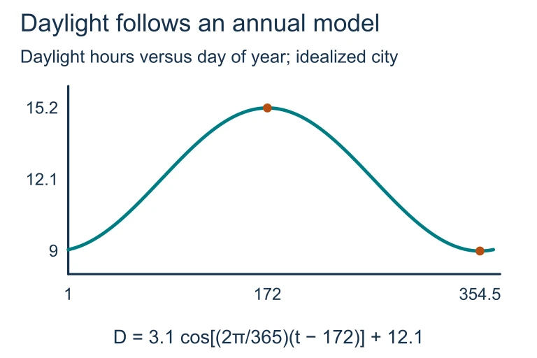
Substituting all parameters: D(t) = 3.1 cos((2π/365)(t − 172)) + 12.1. Verification: D(172) = 3.1 cos(0) + 12.1 = 3.1(1) + 12.1 = 15.2 ✓. Check the minimum: D(355) = 3.1 cos((2π/365)(355 − 172)) + 12.1 = 3.1 cos((2π/365)(183)) + 12.1 ≈ 3.1 cos(π) + 12.1 = 3.1(−1) + 12.1 = 9.0 ✓.

D(t) = 3.1 cos((2π/365)(t − 172)) + 12.1

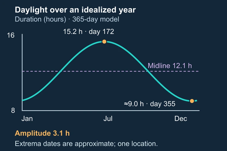Annual daylight model with midpoint 12.1 hours, amplitude 3.1 hours, maximum 15.2 near day 172 and minimum near 9 hours around day 355. The seasonal scenes share one location; exact duration bars show the approximate extrema of the stated 365-day daylight model.

This example demonstrates the power of the cosine form: by aligning the phase shift with the known maximum, we avoid having to locate a midline crossing. The verification step is essential — always check that your model reproduces the known extremes. Note that 183 days is approximately half of 365, making (2π/365)(183) ≈ π, which confirms that the minimum is half a period away from the maximum, as expected for a symmetric sinusoidal curve.

Two matched harbor views show the same fixed pier, pilings, shoreline buildings and blue boat at higher water and lower water; exposed rocks and piling lengths increase in the lower-water view. The harbor scene introduces periodic change; the accompanying graph models annual daylight. Annual daylight has midline 12.1 hours, amplitude 3.1 hours, and period 365 days. Its maximum occurs at day 172.

The harbor scene introduces periodic change; the accompanying graph models annual daylight. Annual daylight has midline 12.1 hours, amplitude 3.1 hours, and period 365 days. Its maximum occurs at day 172.

SECTION 7

Strengths, Limitations & Model Assumptions

Every mathematical model carries assumptions, and the sinusoidal model is no exception. Understanding both its strengths and its limitations helps you assess when a sinusoidal function is the best choice and when an alternative model — such as a piecewise function, exponential decay, or Fourier series — might be more appropriate. The table below summarizes the key tradeoffs.

Feature	Strength	Limitation
Periodicity	Perfectly captures repeating cycles of constant length.	Cannot model phenomena whose cycle length changes over time (e.g., accelerating heartbeat).
Symmetry	Rise and fall times are equal — ideal for many natural cycles.	Fails when the rise is fast and the fall is slow (e.g., sawtooth waves in electronics).
Smoothness	Infinitely differentiable — excellent for approximation and calculus applications.	Cannot model sharp discontinuities or abrupt regime changes.
Simplicity	Only four parameters — easy to interpret and communicate.	May oversimplify complex oscillations that require multiple harmonics.
Extrapolation	Can predict future values as long as the periodic pattern persists.	Assumes stationarity — does not account for trends (e.g., global warming shifting the midline).

Strengths and limitations of the sinusoidal model

✦

KEY TAKEAWAY

A sinusoidal model is like a perfectly balanced pendulum: it swings symmetrically and tirelessly at a fixed rate. Real-world data is more like a pendulum in a windstorm — it may drift, wobble, or slow down. The sinusoidal model works best when the dominant behavior of the data is periodic and symmetric; non-periodic trends or asymmetric oscillations require more sophisticated tools such as Fourier series or piecewise models.

SECTION 8

Connections to Advanced Theory

The sinusoidal functions you master in AP Precalculus form the foundation for several advanced topics that you will encounter in calculus, physics, and engineering. This section briefly outlines how the ideas in this lesson connect forward, giving you a roadmap for deeper study.

AP Precalculus Concept	Advanced Extension	Where You'll See It
Single sinusoidal model f(x) = a sin(b(x − c)) + d	Fourier series: any periodic function as an infinite sum of sinusoids	Multivariable calculus, signal processing, physics of waves
Amplitude and period from context	Damped oscillations: amplitude decays exponentially over time (ae⁻ᵏᵗ sin(ωt))	Differential equations, mechanical engineering (spring systems)
Phase shift c	Wave interference: phase differences cause constructive/destructive superposition	AP Physics, acoustics, optics, quantum mechanics
Sinusoidal regression from data	Least-squares fitting and spectral analysis for complex data sets	Statistics, data science, climate modeling

How AP Precalculus sinusoidal concepts extend to advanced coursework

In AP Calculus, you will differentiate and integrate sinusoidal functions, discovering that the derivative of sin(x) is cos(x) and vice versa — a relationship that explains why velocity and acceleration in circular motion are themselves sinusoidal. In physics, two waves with different phase shifts combine to form interference patterns, and the mathematics of phase that you learn here directly transfers to understanding standing waves and beats. The four-parameter sinusoidal model is thus not just a curve-fitting tool; it is the entry point into a vast and interconnected web of mathematical and scientific ideas.

SECTION 9

Practice Problems

Question 1: CONCEPTUAL

A scientist records that a certain quantity oscillates between a maximum value of 80 and a minimum value of 20 over a repeating cycle. If a sinusoidal function is used to model this quantity, what are the midline and amplitude of the function?

A. Midline = 40, Amplitude = 20
B. Midline = 50, Amplitude = 30
C. Midline = 50, Amplitude = 60
D. Midline = 60, Amplitude = 20
E. Midline = 30, Amplitude = 50

Show answer (B)

The midline d = (max + min)/2 = (80 + 20)/2 = 50, and the amplitude |a| = (max − min)/2 = (80 − 20)/2 = 30. Choice A incorrectly computes the midline as half the maximum. Choice C uses the full range (60) instead of half the range for the amplitude. Choice D incorrectly computes the midline and amplitude. Choice E reverses the formulas, placing the half-difference as midline and the average as amplitude.

Question 2: BASIC CALCULATION

The depth of water in a harbor, in meters, is modeled by D(t) = 4.5 sin((π/6)(t − 3)) + 8, where t is measured in hours after midnight. What is the period of the tide cycle, and at what time does the first maximum depth occur?

A. Period = 6 hours; first maximum at t = 3
B. Period = 12 hours; first maximum at t = 3
C. Period = 12 hours; first maximum at t = 6
D. Period = 12 hours; first maximum at t = 9
E. Period = 24 hours; first maximum at t = 6

Show answer (C)

The period T = 2π/|b| = 2π/(π/6) = 12 hours. The sine function reaches its maximum when its argument equals π/2. Setting (π/6)(t − 3) = π/2 gives t − 3 = 3, so t = 6 (6:00 AM). Choice A incorrectly computes the period as 2π/π × 1 = 6. Choice B identifies t = 3 as the maximum, but at t = 3 the sine argument is 0, giving D = 8 (midline, not maximum). Choice D adds a full quarter-period to the wrong reference. Choice E uses T = 24 hours, which would require b = π/12, not π/6.

Question 3: INTERMEDIATE

The average monthly temperature in a city ranges from a low of 28°F in January (month 1) to a high of 84°F in July (month 7). A student writes the model T(m) = −28 cos((π/6)(m − 1)) + 56. A classmate claims this model is incorrect. Which of the following statements about the model is true?

A. The amplitude should be 56, not 28, because the temperature range is 84 − 28 = 56.
B. The model is correct: the negative cosine reaches its minimum at m = 1, giving T(1) = 56 − 28 = 28°F, and its maximum at m = 7, giving T(7) = 56 + 28 = 84°F.
C. The negative sign is wrong; it should be positive because cosine starts at its maximum.
D. The phase shift should be 7 instead of 1 because the maximum occurs in month 7.
E. The frequency factor should give a period of 6 months, not 12, because there are only 6 months between the max and min.

Show answer (B)

Checking the original model T(m) = −28 cos((π/6)(m − 1)) + 56: At m = 1, T(1) = −28 cos(0) + 56 = −28 + 56 = 28°F ✓. At m = 7, T(7) = −28 cos(π) + 56 = 28 + 56 = 84°F ✓. The period is 2π/(π/6) = 12 months ✓. The midline is (84 + 28)/2 = 56 ✓. The amplitude is (84 − 28)/2 = 28 ✓. The model is fully correct. Choice A confuses the full range (56) with the amplitude (28). Choice C misidentifies the role of the negative sign — with a negative cosine the minimum aligns with the phase shift, so c = 1 correctly places the minimum at January. Choice D incorrectly claims the phase shift should be 7 to align with the maximum, but the negative cosine naturally places the maximum half a period away from the phase shift. Choice E incorrectly states that the period is wrong because there are only 6 months between max and min — 6 months is half the period, so the full period of 12 months is correct.

Question 4: APPLIED

4 pts

A Ferris wheel has a diameter of 40 meters, and its center is 25 meters above the ground. The wheel completes one revolution every 8 minutes. A rider boards at the lowest point of the wheel at time t = 0 minutes. (a) Write a sinusoidal function H(t) that gives the rider's height above the ground as a function of time t in minutes. (b) Find the height of the rider at t = 3 minutes. (c) Determine all times during the first revolution when the rider is exactly 35 meters above the ground. (d) A second rider boards 2 minutes after the first. Write a function H₂(t) for the second rider's height, using the same time variable t.

Show answer

Rubric (4 points): (a) [1 point] The radius is 20 m, so a = 20. The midline is d = 25. The period is T = 8, so b = 2π/8 = π/4. Since the rider starts at the lowest point (minimum), use a negative cosine: H(t) = −20 cos((π/4)t) + 25. Award 1 point for a correct function with appropriate amplitude, period, midline, and phase/reflection that yields H(0) = 5. (b) [1 point] H(3) = −20 cos((π/4)(3)) + 25 = −20 cos(3π/4) + 25 = −20(−√2/2) + 25 = 10√2 + 25 ≈ 39.14 meters. Award 1 point for correct substitution and simplification. (c) [1 point] Set 35 = −20 cos((π/4)t) + 25 → −20 cos((π/4)t) = 10 → cos((π/4)t) = −1/2. So (π/4)t = 2π/3 or (π/4)t = 4π/3, giving t = 8/3 ≈ 2.67 minutes and t = 16/3 ≈ 5.33 minutes. Award 1 point for both correct times with valid supporting work. (d) [1 point] The second rider boards at t = 2 at the lowest point, so replace t with (t − 2): H₂(t) = −20 cos((π/4)(t − 2)) + 25. Award 1 point for the correct horizontal shift that produces H₂(2) = 5.

Question 5: CRITICAL THINKING

3 pts

A researcher collects the following data on the average daily temperature (°F) for a coastal city: Month 1: 52, Month 4: 63, Month 7: 78, Month 10: 67, Month 13: 53 (a) Using the data, determine whether a sinusoidal model is appropriate. Justify your answer. (b) The researcher notices that the maximum temperature occurs closer to month 8 than month 7 for the actual data. Explain how this observation affects the phase shift parameter and write the adjusted cosine model. (c) Predict the temperature at month 19 using your model from part (b). Interpret this prediction in context.

Show answer

Rubric (3 points): (a) [1 point] The data rises from 52 to 78 and falls back to 53 over approximately 12 months, indicating periodic behavior. The rise (months 1–7) and fall (months 7–13) are roughly symmetric. The values oscillate between about 52 and 78 with no apparent trend. These three conditions — periodicity, symmetry, and boundedness — justify a sinusoidal model. Award 1 point for citing at least two of these conditions with supporting evidence from the data. (b) [1 point] With the maximum shifted to month 8, the phase shift becomes c = 8 instead of c = 7. Using d = (78 + 52)/2 = 65, |a| = (78 − 52)/2 = 13, T = 12, b = 2π/12 = π/6: T(m) = 13 cos((π/6)(m − 8)) + 65. Award 1 point for a correct adjusted model with c = 8 and all other parameters correctly computed. (c) [1 point] T(19) = 13 cos((π/6)(19 − 8)) + 65 = 13 cos(11π/6) + 65 = 13(√3/2) + 65 ≈ 11.26 + 65 ≈ 76.3°F. Since month 19 corresponds to month 7 of the second year (July), this prediction of approximately 76°F is consistent with a summer temperature slightly below the peak, which makes contextual sense because month 19 is one month before the annual maximum at month 20 (= 8 + 12). Award 1 point for a correct computation with a contextual interpretation.

SUMMARY

Lesson Summary

Summary

A sinusoidal function of the form f(x) = a sin(b(x − c)) + d or f(x) = a cos(b(x − c)) + d is characterized by four parameters: the amplitude |a| (half the range), the period T = 2π/|b| (length of one cycle), the phase shift c (horizontal translation), and the midline d (average value). To model real-world data, compute the midline as d = (max + min)/2, the amplitude as |a| = (max − min)/2, the frequency factor as b = 2π/T, and the phase shift by locating a maximum (cosine form) or midline crossing (sine form).

A sinusoidal model is appropriate when data exhibits periodicity, symmetry, and boundedness. Its limitations include the assumption of constant period, symmetric oscillation, and no long-term trend. Always validate your model by substituting known data points back into the function. The sinusoidal model is the gateway to Fourier analysis, damped oscillations, and wave interference — advanced concepts that build directly on the four-parameter framework mastered here.